Example 30 - Planar Dipping Layers

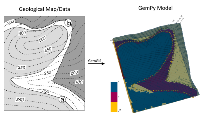
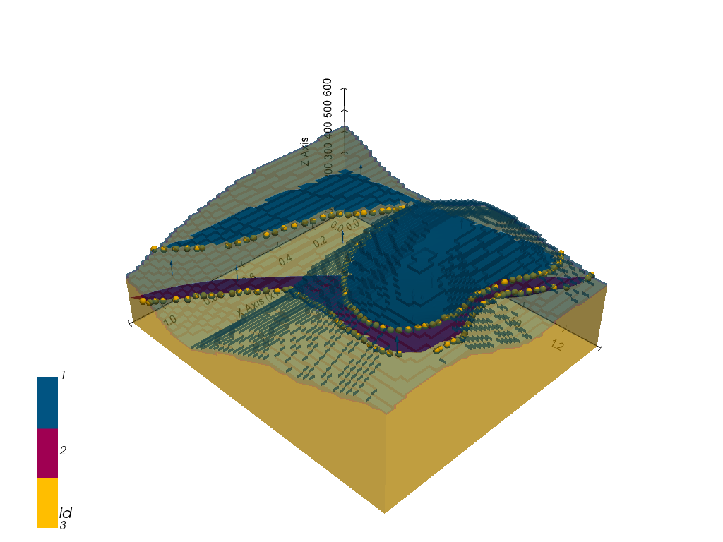
This example will show how to convert the geological map below using GemGIS to a GemPy model. This example is based on digitized data. The area is 1157 m wide (W-E extent) and 1361 m high (N-S extent). The vertical model extents varies between 0 m and 600 m. The model represents two planar stratigraphic units (blue and red) dipping towards the northeast above an unspecified basement (yellow). The map has been georeferenced with QGIS. The stratigraphic boundaries were digitized in QGIS. Strikes lines were digitized in QGIS as well and were used to calculate orientations for the GemPy model. These will be loaded into the model directly. The contour lines were also digitized and will be interpolated with GemGIS to create a topography for the model.

Map Source: Unknown

import matplotlib.pyplot as plt
import matplotlib.image as mpimg
img = mpimg.imread('../images/cover_example30.png')
plt.figure(figsize=(10, 10))
imgplot = plt.imshow(img)
plt.axis('off')
plt.tight_layout()

Licensing

Computational Geosciences and Reservoir Engineering, RWTH Aachen University, Authors: Alexander Juestel. For more information contact: alexander.juestel(at)rwth-aachen.de

This work is licensed under a Creative Commons Attribution 4.0 International License (http://creativecommons.org/licenses/by/4.0/)

Import GemGIS

If you have installed GemGIS via pip or conda, you can import GemGIS like any other package. If you have downloaded the repository, append the path to the directory where the GemGIS repository is stored and then import GemGIS.

import warnings
warnings.filterwarnings("ignore")
import gemgis as gg

Importing Libraries and loading Data

All remaining packages can be loaded in order to prepare the data and to construct the model. The example data is downloaded from an external server using pooch. It will be stored in a data folder in the same directory where this notebook is stored.

import geopandas as gpd
import rasterio

file_path = 'data/example30/'
gg.download_gemgis_data.download_tutorial_data(filename="example30_planar_dipping_layers.zip", dirpath=file_path)

Downloading file 'example30_planar_dipping_layers.zip' from 'https://rwth-aachen.sciebo.de/s/AfXRsZywYDbUF34/download?path=%2Fexample30_planar_dipping_layers.zip' to 'C:\Users\ale93371\Documents\gemgis\docs\getting_started\example\data\example30'.

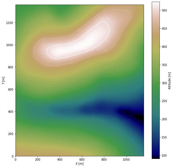
Creating Digital Elevation Model from Contour Lines

The digital elevation model (DEM) will be created by interpolating contour lines digitized from the georeferenced map using the SciPy Radial Basis Function interpolation wrapped in GemGIS. The respective function used for that is gg.vector.interpolate_raster().

import matplotlib.pyplot as plt
import matplotlib.image as mpimg
img = mpimg.imread('../images/dem_example30.png')
plt.figure(figsize=(10, 10))
imgplot = plt.imshow(img)
plt.axis('off')
plt.tight_layout()

topo = gpd.read_file(file_path + 'topo30.shp')
topo.head()

	id	Z	geometry
0	None	400	LINESTRING (4.295 91.552, 43.424 86.924, 83.39...
1	None	350	LINESTRING (3.874 182.012, 64.462 176.122, 125...
2	None	300	LINESTRING (4.716 300.242, 37.534 286.357, 86....
3	None	100	LINESTRING (1156.295 265.320, 1138.203 282.570...
4	None	300	LINESTRING (1.771 1206.526, 24.912 1231.771, 4...

Interpolating the contour lines

topo_raster = gg.vector.interpolate_raster(gdf=topo, value='Z', method='rbf', res=10)

Plotting the raster

import matplotlib.pyplot as plt

fix, ax = plt.subplots(1, figsize=(10, 10))
topo.plot(ax=ax, aspect='equal', column='Z', cmap='gist_earth')
im = plt.imshow(topo_raster, origin='lower', extent=[0, 1157, 0, 1361], cmap='gist_earth')
cbar = plt.colorbar(im)
cbar.set_label('Altitude [m]')
plt.xlabel('X [m]')
plt.ylabel('Y [m]')
plt.xlim(0, 1157)
plt.ylim(0, 1361)

(0.0, 1361.0)

Saving the raster to disc

After the interpolation of the contour lines, the raster is saved to disc using gg.raster.save_as_tiff(). The function will not be executed as a raster is already provided with the example data.

gg.raster.save_as_tiff(raster=topo_raster, path=file_path + 'raster30.tif', extent=[0, 1157, 0, 1361], crs='EPSG:4326', overwrite_file=True)

Opening Raster

The previously computed and saved raster can now be opened using rasterio.

topo_raster = rasterio.open(file_path + 'raster30.tif')

Interface Points of stratigraphic boundaries

The interface points will be extracted from LineStrings digitized from the georeferenced map using QGIS. It is important to provide a formation name for each layer boundary. The vertical position of the interface point will be extracted from the digital elevation model using the GemGIS function gg.vector.extract_xyz(). The resulting GeoDataFrame now contains single points including the information about the respective formation.

img = mpimg.imread('../images/interfaces_example30.png')
plt.figure(figsize=(10, 10))
imgplot = plt.imshow(img)
plt.axis('off')
plt.tight_layout()

interfaces = gpd.read_file(file_path + 'interfaces30.shp')
interfaces.head()

	id	formation	geometry
0	None	A	LINESTRING (1003.775 4.248, 979.792 33.489, 94...
1	None	B	LINESTRING (2.612 1272.583, 33.747 1279.105, 1...

Extracting Z coordinate from Digital Elevation Model

interfaces_coords = gg.vector.extract_xyz(gdf=interfaces, dem=topo_raster)
interfaces_coords = interfaces_coords[interfaces_coords['formation'].isin(['A', 'B'])]
interfaces_coords

	formation	geometry	X	Y	Z
0	A	POINT (1003.775 4.248)	1003.77	4.25	274.58
1	A	POINT (979.792 33.489)	979.79	33.49	276.06
2	A	POINT (949.919 67.149)	949.92	67.15	280.72
3	A	POINT (919.626 97.232)	919.63	97.23	282.11
4	A	POINT (891.226 121.425)	891.23	121.43	279.32
...	...	...	...	...	...
178	B	POINT (1065.624 207.047)	1065.62	207.05	178.74
179	B	POINT (1102.019 177.174)	1102.02	177.17	176.01
180	B	POINT (1121.373 159.713)	1121.37	159.71	175.79
181	B	POINT (1139.255 144.987)	1139.25	144.99	170.98
182	B	POINT (1155.664 128.367)	1155.66	128.37	176.47

183 rows × 5 columns

Plotting the Interface Points

fig, ax = plt.subplots(1, figsize=(10, 10))

interfaces.plot(ax=ax, column='formation', legend=True, aspect='equal')
interfaces_coords.plot(ax=ax, column='formation', legend=True, aspect='equal')
plt.grid()
plt.xlabel('X [m]')
plt.ylabel('Y [m]')
plt.xlim(0, 1157)
plt.ylim(0, 1361)

(0.0, 1361.0)

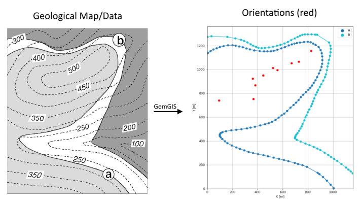
Orientations from Strike Lines

Strike lines connect outcropping stratigraphic boundaries (interfaces) of the same altitude. In other words: the intersections between topographic contours and stratigraphic boundaries at the surface. The height difference and the horizontal difference between two digitized lines is used to calculate the dip and azimuth and hence an orientation that is necessary for GemPy. In order to calculate the orientations, each set of strikes lines/LineStrings for one formation must be given an id number next to the altitude of the strike line. The id field is already predefined in QGIS. The strike line with the lowest altitude gets the id number 1, the strike line with the highest altitude the the number according to the number of digitized strike lines. It is currently recommended to use one set of strike lines for each structural element of one formation as illustrated.

img = mpimg.imread('../images/orientations_example30.png')
plt.figure(figsize=(10, 10))
imgplot = plt.imshow(img)
plt.axis('off')
plt.tight_layout()

strikes = gpd.read_file(file_path + 'strikes30.shp')
strikes

	id	formation	Z	geometry
0	5	A	450	LINESTRING (672.648 1212.207, 908.266 1026.237)
1	4	A	400	LINESTRING (488.362 1152.461, 840.105 873.928)
2	3	A	350	LINESTRING (155.132 1200.426, 738.285 759.485)
3	7	B	450	LINESTRING (981.475 1168.449, 790.457 1296.356)
4	6	B	400	LINESTRING (936.876 944.613, 586.816 1212.207)
5	5	B	350	LINESTRING (872.923 809.133, 275.465 1250.915)
6	4	B	300	LINESTRING (837.581 713.203, 103.801 1281.209)
7	2	A	300	LINESTRING (595.231 618.115, -48.508 1111.228)
8	1	A	250	LINESTRING (104.643 462.439, -276.552 771.266)
9	3	B	250	LINESTRING (790.457 620.639, 47.421 1186.120)
10	2	B	200	LINESTRING (749.224 524.709, -58.606 1140.680)
11	1	B	150	LINESTRING (765.212 382.497, 12.079 963.125)

Calculating Orientations for each formation

orientations_a = gg.vector.calculate_orientations_from_strike_lines(gdf=strikes[strikes['formation'] == 'A'].sort_values(by='id', ascending=True).reset_index())
orientations_a

	dip	azimuth	Z	geometry	polarity	formation	X	Y
0	6.98	217.87	275.00	POINT (93.703 740.762)	1.00	A	93.70	740.76
1	14.41	217.29	325.00	POINT (360.035 922.313)	1.00	A	360.03	922.31
2	18.11	217.45	375.00	POINT (555.471 996.575)	1.00	A	555.47	996.57
3	17.23	218.35	425.00	POINT (727.345 1066.208)	1.00	A	727.35	1066.21

orientations_b = gg.vector.calculate_orientations_from_strike_lines(gdf=strikes[strikes['formation'] == 'B'].sort_values(by='id', ascending=True).reset_index())
orientations_b

	dip	azimuth	Z	geometry	polarity	formation	X	Y
0	26.95	217.47	175.00	POINT (366.977 752.753)	1.00	B	366.98	752.75
1	26.47	217.30	225.00	POINT (382.124 868.037)	1.00	B	382.12	868.04
2	26.07	217.51	275.00	POINT (444.815 950.293)	1.00	B	444.82	950.29
3	31.65	217.25	325.00	POINT (522.443 1013.615)	1.00	B	522.44	1013.61
4	18.79	216.72	375.00	POINT (668.020 1054.217)	1.00	B	668.02	1054.22
5	14.70	216.63	425.00	POINT (823.906 1155.406)	1.00	B	823.91	1155.41

Merging Orientations

import pandas as pd
orientations = pd.concat([orientations_a, orientations_b])
orientations = orientations[orientations['formation'].isin(['A', 'B'])].reset_index()
orientations

	index	dip	azimuth	Z	geometry	polarity	formation	X	Y
0	0	6.98	217.87	275.00	POINT (93.703 740.762)	1.00	A	93.70	740.76
1	1	14.41	217.29	325.00	POINT (360.035 922.313)	1.00	A	360.03	922.31
2	2	18.11	217.45	375.00	POINT (555.471 996.575)	1.00	A	555.47	996.57
3	3	17.23	218.35	425.00	POINT (727.345 1066.208)	1.00	A	727.35	1066.21
4	0	26.95	217.47	175.00	POINT (366.977 752.753)	1.00	B	366.98	752.75
5	1	26.47	217.30	225.00	POINT (382.124 868.037)	1.00	B	382.12	868.04
6	2	26.07	217.51	275.00	POINT (444.815 950.293)	1.00	B	444.82	950.29
7	3	31.65	217.25	325.00	POINT (522.443 1013.615)	1.00	B	522.44	1013.61
8	4	18.79	216.72	375.00	POINT (668.020 1054.217)	1.00	B	668.02	1054.22
9	5	14.70	216.63	425.00	POINT (823.906 1155.406)	1.00	B	823.91	1155.41

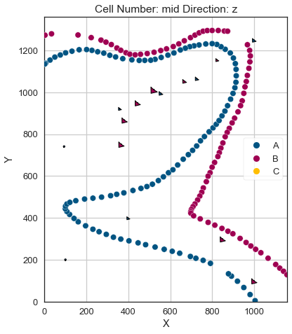
Plotting the Orientations

fig, ax = plt.subplots(1, figsize=(10, 10))

interfaces.plot(ax=ax, column='formation', legend=True, aspect='equal')
interfaces_coords.plot(ax=ax, column='formation', legend=True, aspect='equal')
orientations.plot(ax=ax, color='red', aspect='equal')
plt.grid()
plt.xlabel('X [m]')
plt.ylabel('Y [m]')
plt.xlim(0, 1157)
plt.ylim(0, 1361)

(0.0, 1361.0)

GemPy Model Construction

The structural geological model will be constructed using the GemPy package.

import gempy as gp

WARNING (theano.configdefaults): g++ not available, if using conda: `conda install m2w64-toolchain`
WARNING (theano.configdefaults): g++ not detected ! Theano will be unable to execute optimized C-implementations (for both CPU and GPU) and will default to Python implementations. Performance will be severely degraded. To remove this warning, set Theano flags cxx to an empty string.
WARNING (theano.tensor.blas): Using NumPy C-API based implementation for BLAS functions.

Creating new Model

geo_model = gp.create_model('Model30')
geo_model

Model30  2022-04-17 08:51

Initiate Data

gp.init_data(geo_model, [0, 1157, 0, 1361, 0, 600], [50,50,50],
             surface_points_df=interfaces_coords,
             orientations_df=orientations,
             default_values=True)

Active grids: ['regular']

Model30  2022-04-17 08:51

Model Surfaces

geo_model.surfaces

	surface	series	order_surfaces	color	id
0	A	Default series	1	#015482	1
1	B	Default series	2	#9f0052	2

Mapping the Stack to Surfaces

gp.map_stack_to_surfaces(geo_model,
                         {'Strata1': ('A'),
                          'Strata2': ('B')
                         },
                         remove_unused_series=True)
geo_model.add_surfaces('C')

	surface	series	order_surfaces	color	id
0	A	Strata1	1	#015482	1
1	B	Strata2	1	#9f0052	2
2	C	Strata2	2	#ffbe00	3

Adding additional orientations

geo_model.add_orientations(X=1000, Y=1250, Z=500, surface='A', orientation = [217.5,18,1])
geo_model.add_orientations(X=100, Y=200, Z=300, surface='A', orientation = [217.5,7,1])
geo_model.add_orientations(X=400, Y=400, Z=200, surface='A', orientation = [217.5,14.5,1])

geo_model.add_orientations(X=850, Y=300, Z=200, surface='B', orientation = [217.5,26,1])
geo_model.add_orientations(X=1000, Y=100, Z=200, surface='B', orientation = [217.5,26,1])

	X	Y	Z	G_x	G_y	G_z	smooth	surface
0	93.70	740.76	275.00	-0.07	-0.10	0.99	0.01	A
1	360.03	922.31	325.00	-0.15	-0.20	0.97	0.01	A
2	555.47	996.57	375.00	-0.19	-0.25	0.95	0.01	A
3	727.35	1066.21	425.00	-0.18	-0.23	0.96	0.01	A
10	1000.00	1250.00	500.00	-0.19	-0.25	0.95	0.01	A
11	100.00	200.00	300.00	-0.07	-0.10	0.99	0.01	A
12	400.00	400.00	200.00	-0.15	-0.20	0.97	0.01	A
4	366.98	752.75	175.00	-0.28	-0.36	0.89	0.01	B
5	382.12	868.04	225.00	-0.27	-0.35	0.90	0.01	B
6	444.82	950.29	275.00	-0.27	-0.35	0.90	0.01	B
7	522.44	1013.61	325.00	-0.32	-0.42	0.85	0.01	B
8	668.02	1054.22	375.00	-0.19	-0.26	0.95	0.01	B
9	823.91	1155.41	425.00	-0.15	-0.20	0.97	0.01	B
13	850.00	300.00	200.00	-0.27	-0.35	0.90	0.01	B
14	1000.00	100.00	200.00	-0.27	-0.35	0.90	0.01	B

Showing the Number of Data Points

gg.utils.show_number_of_data_points(geo_model=geo_model)

	surface	series	order_surfaces	color	id	No. of Interfaces	No. of Orientations
0	A	Strata1	1	#015482	1	102	7
1	B	Strata2	1	#9f0052	2	81	8
2	C	Strata2	2	#ffbe00	3	0	0

Loading Digital Elevation Model

geo_model.set_topography(source='gdal', filepath=file_path + 'raster30.tif')

Cropped raster to geo_model.grid.extent.
depending on the size of the raster, this can take a while...
storing converted file...
Active grids: ['regular' 'topography']

Grid Object. Values:
array([[  11.57      ,   13.61      ,    6.        ],
       [  11.57      ,   13.61      ,   18.        ],
       [  11.57      ,   13.61      ,   30.        ],
       ...,
       [1152.01293103, 1335.98161765,  415.3067627 ],
       [1152.01293103, 1345.98897059,  416.07495117],
       [1152.01293103, 1355.99632353,  416.66900635]])

Plotting Input Data

gp.plot_2d(geo_model, direction='z', show_lith=False, show_boundaries=False)
plt.grid()

gp.plot_3d(geo_model, image=False, plotter_type='basic', notebook=True)

<gempy.plot.vista.GemPyToVista at 0x26e9ff0c730>

Setting the Interpolator

gp.set_interpolator(geo_model,
                    compile_theano=True,
                    theano_optimizer='fast_compile',
                    verbose=[],
                    update_kriging=False
                    )

Compiling theano function...
Level of Optimization:  fast_compile
Device:  cpu
Precision:  float64
Number of faults:  0
Compilation Done!
Kriging values:
                  values
range            1884.4
$C_o$           84546.9
drift equations  [3, 3]

<gempy.core.interpolator.InterpolatorModel at 0x26ea597b7f0>

Computing Model

sol = gp.compute_model(geo_model, compute_mesh=True)

Plotting Cross Sections

gp.plot_2d(geo_model, direction=['x', 'x', 'y', 'y'], cell_number=[25, 40, 25, 40], show_topography=True, show_data=False)

<gempy.plot.visualization_2d.Plot2D at 0x26eaf241040>

gpv = gp.plot_3d(geo_model, image=False, show_topography=False,
                 plotter_type='basic', notebook=True, show_lith=True)