
Example 2 - Planar Dipping Layers
Contents
Example 2 - Planar Dipping Layers#
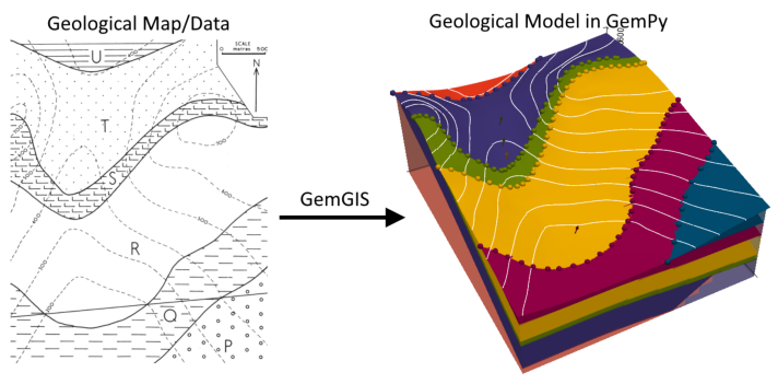
This example will show how to convert the geological map below using GemGIS to a GemPy model. This example is based on digitized data. The area is 2932 m wide (W-E extent) and 3677 m high (N-S extent). The vertical model extent varies between -700 m and 1000 m. The model represents several planar stratigraphic units (blue to purple) dipping towards the south above an unspecified basement (light red). The map has been georeferenced with QGIS. The stratigraphic boundaries were digitized in
QGIS. Strikes lines were digitized in QGIS as well and will be used to calculate orientations for the GemPy model. The contour lines were also digitized and will be interpolated with GemGIS to create a topography for the model.
Map Source: An Introduction to Geological Structures and Maps by G.M. Bennison
[1]:
import matplotlib.pyplot as plt
import matplotlib.image as mpimg
img = mpimg.imread('../images/cover_example02.png')
plt.figure(figsize=(10, 10))
imgplot = plt.imshow(img)
plt.axis('off')
plt.tight_layout()
Licensing#
Computational Geosciences and Reservoir Engineering, RWTH Aachen University, Authors: Alexander Juestel. For more information contact: alexander.juestel(at)rwth-aachen.de
This work is licensed under a Creative Commons Attribution 4.0 International License (http://creativecommons.org/licenses/by/4.0/)
Import GemGIS#
If you have installed GemGIS via pip or conda, you can import GemGIS like any other package. If you have downloaded the repository, append the path to the directory where the GemGIS repository is stored and then import GemGIS.
[2]:
import warnings
warnings.filterwarnings("ignore")
import gemgis as gg
Importing Libraries and loading Data#
All remaining packages can be loaded in order to prepare the data and to construct the model. The example data is downloaded from an external server using pooch. It will be stored in a data folder in the same directory where this notebook is stored.
[3]:
import geopandas as gpd
import rasterio
[4]:
file_path = '../data/example02/'
gg.download_gemgis_data.download_tutorial_data(filename="example02_planar_dipping_layers.zip", dirpath=file_path)
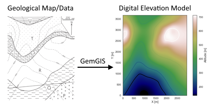
Creating Digital Elevation Model from Contour Lines#
The digital elevation model (DEM) will be created by interpolating contour lines digitized from the georeferenced map using the SciPy Radial Basis Function interpolation wrapped in GemGIS. The respective function used for that is gg.vector.interpolate_raster().
[5]:
import matplotlib.pyplot as plt
import matplotlib.image as mpimg
img = mpimg.imread('../images/dem_example2.png')
plt.figure(figsize=(10, 10))
imgplot = plt.imshow(img)
plt.axis('off')
plt.tight_layout()
[6]:
topo = gpd.read_file(file_path + 'topo2.shp')
topo.head()
[6]:
| id | Z | geometry | |
|---|---|---|---|
| 0 | None | 200 | LINESTRING (66.248 9.085, 187.630 201.563, 284... |
| 1 | None | 300 | LINESTRING (2.089 534.498, 109.599 713.104, 22... |
| 2 | None | 400 | LINESTRING (5.557 1167.421, 69.716 1294.006, 1... |
| 3 | None | 700 | LINESTRING (5.557 2894.521, 59.312 2939.606, 1... |
| 4 | None | 600 | LINESTRING (7.291 3267.338, 69.716 3288.147, 1... |
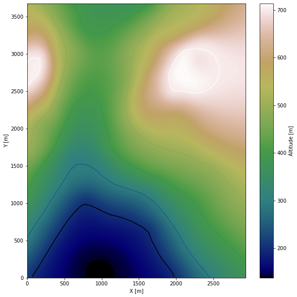
Interpolating the contour lines#
[7]:
topo_raster = gg.vector.interpolate_raster(gdf=topo, value='Z', method='rbf', res=10)
Plotting the raster#
[8]:
import matplotlib.pyplot as plt

fix, ax = plt.subplots(1, figsize=(10, 10))
topo.plot(ax=ax, aspect='equal', column='Z', cmap='gist_earth')
im = plt.imshow(topo_raster, origin='lower', extent=[0, 2932, 0, 3677], cmap='gist_earth')
cbar = plt.colorbar(im)
cbar.set_label('Altitude [m]')
ax.set_xlabel('X [m]')
ax.set_ylabel('Y [m]')
ax.set_xlim(0, 2932)
ax.set_ylim(0, 3677)
[8]:
(0.0, 3677.0)
Saving the raster to disc#
After the interpolation of the contour lines, the raster is saved to disc using gg.raster.save_as_tiff(). The function will not be executed as a raster is already provided with the example data.
Opening Raster#
The previously computed and saved raster can now be opened using rasterio.
[9]:
topo_raster = rasterio.open(file_path + 'raster2.tif')
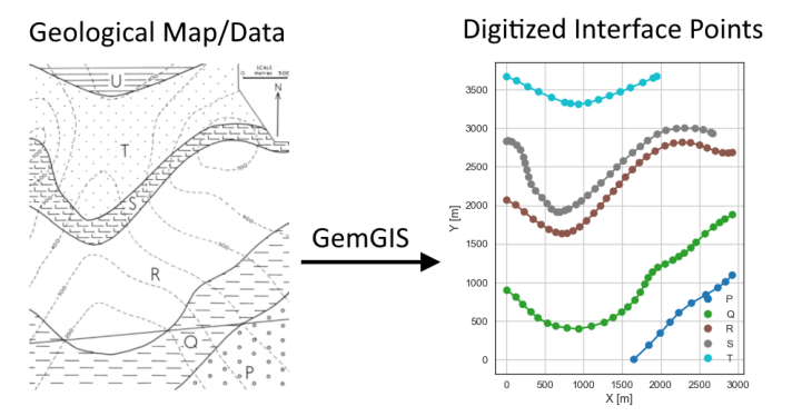
Interface Points of stratigraphic boundaries#
The interface points will be extracted from LineStrings digitized from the georeferenced map using QGIS. It is important to provide a formation name for each layer boundary. The vertical position of the interface point will be extracted from the digital elevation model using the GemGIS function gg.vector.extract_xyz(). The resulting GeoDataFrame now contains single points including the information about the respective formation.
[10]:
import matplotlib.pyplot as plt
import matplotlib.image as mpimg
img = mpimg.imread('../images/interfaces_example2.png')
plt.figure(figsize=(10, 10))
imgplot = plt.imshow(img)
plt.axis('off')
plt.tight_layout()
[11]:
interfaces = gpd.read_file(file_path + 'interfaces2.shp')
interfaces.head()
[11]:
| id | formation | geometry | |
|---|---|---|---|
| 0 | None | P | LINESTRING (1652.891 2.149, 1847.103 185.957, ... |
| 1 | None | Q | LINESTRING (7.291 898.645, 125.205 810.210, 21... |
| 2 | None | R | LINESTRING (5.557 2067.386, 121.737 2004.960, ... |
| 3 | None | S | LINESTRING (4.690 2829.494, 27.232 2837.298, 7... |
| 4 | None | T | LINESTRING (4.690 3667.901, 133.875 3615.013, ... |
Extracting Z coordinate from Digital Elevation Model#
[12]:
interfaces_coords = gg.vector.extract_xyz(gdf=interfaces, dem=topo_raster)
interfaces_coords
[12]:
| formation | geometry | X | Y | Z | |
|---|---|---|---|---|---|
| 0 | P | POINT (1652.891 2.149) | 1652.89 | 2.15 | 162.71 |
| 1 | P | POINT (1847.103 185.957) | 1847.10 | 185.96 | 196.79 |
| 2 | P | POINT (1994.496 342.020) | 1994.50 | 342.02 | 252.93 |
| 3 | P | POINT (2121.080 484.211) | 2121.08 | 484.21 | 305.56 |
| 4 | P | POINT (2235.527 607.327) | 2235.53 | 607.33 | 349.55 |
| ... | ... | ... | ... | ... | ... |
| 121 | T | POINT (1476.886 3471.088) | 1476.89 | 3471.09 | 421.32 |
| 122 | T | POINT (1608.673 3525.710) | 1608.67 | 3525.71 | 436.16 |
| 123 | T | POINT (1768.204 3591.603) | 1768.20 | 3591.60 | 459.65 |
| 124 | T | POINT (1903.459 3650.560) | 1903.46 | 3650.56 | 486.01 |
| 125 | T | POINT (1951.145 3671.369) | 1951.14 | 3671.37 | 490.75 |
126 rows × 5 columns
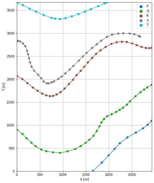
Plotting the Interface Points#
[13]:
fig, ax = plt.subplots(1, figsize=(10, 10))

interfaces.plot(ax=ax, column='formation', legend=True, aspect='equal')
interfaces_coords.plot(ax=ax, column='formation', legend=True, aspect='equal')
plt.grid()
ax.set_xlabel('X [m]')
ax.set_ylabel('Y [m]')
ax.set_xlim(0, 2932)
ax.set_ylim(0, 3677)
[13]:
(0.0, 3677.0)
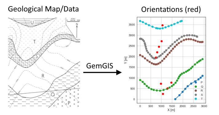
Orientations from Strike Lines#
Strike lines connect outcropping stratigraphic boundaries (interfaces) of the same altitude. In other words: the intersections between topographic contours and stratigraphic boundaries at the surface. The height difference and the horizontal difference between two digitized lines is used to calculate the dip and azimuth and hence an orientation that is necessary for GemPy. In order to calculate the orientations, each set of strikes lines/LineStrings for one formation must be given an id
number next to the altitude of the strike line. The id field is already predefined in QGIS. The strike line with the lowest altitude gets the id number 1, the strike line with the highest altitude the the number according to the number of digitized strike lines. It is currently recommended to use one set of strike lines for each structural element of one formation as illustrated.
[14]:
import matplotlib.pyplot as plt
import matplotlib.image as mpimg
img = mpimg.imread('../images/orientations_example2.png')
plt.figure(figsize=(10, 10))
imgplot = plt.imshow(img)
plt.axis('off')
plt.tight_layout()
[15]:
strikes = gpd.read_file(file_path + 'strikes2.shp')
strikes
[15]:
| id | formation | Z | geometry | |
|---|---|---|---|---|
| 0 | 1 | Q | 200 | LINESTRING (399.616 550.104, 1562.287 669.319) |
| 1 | 2 | Q | 300 | LINESTRING (155.551 778.563, 1774.273 938.095) |
| 2 | 1 | R | 400 | LINESTRING (383.576 1797.309, 1101.467 1861.469) |
| 3 | 2 | R | 500 | LINESTRING (99.195 2015.798, 1347.700 2138.915) |
| 4 | 1 | S | 400 | LINESTRING (503.225 2054.380, 1035.140 2108.569) |
| 5 | 2 | S | 500 | LINESTRING (322.018 2272.002, 1329.493 2383.847) |
| 6 | 3 | S | 600 | LINESTRING (249.189 2524.304, 1626.013 2671.697) |
| 7 | 4 | S | 700 | LINESTRING (155.551 2755.798, 2006.634 2942.207) |
| 8 | 1 | T | 400 | LINESTRING (798.965 3326.642, 1129.884 3348.947) |
| 9 | 2 | T | 500 | LINESTRING (296.896 3529.200, 1983.810 3693.066) |
| 10 | 4 | P | 500 | LINESTRING (2881.434 1048.444, 154.424 778.065) |
| 11 | 3 | P | 400 | LINESTRING (2417.145 743.471, 399.313 550.928) |
| 12 | 2 | P | 300 | LINESTRING (2101.703 460.346, 239.088 291.017) |
| 13 | 1 | P | 200 | LINESTRING (1854.082 194.518, 87.967 44.308) |
Calculate Orientations for each formation#
[16]:
orientations_p = gg.vector.calculate_orientations_from_strike_lines(gdf=strikes[strikes['formation'] == 'P'].sort_values(by='id', ascending=True).reset_index())
orientations_p
[16]:
| dip | azimuth | Z | geometry | polarity | formation | X | Y | |
|---|---|---|---|---|---|---|---|---|
| 0 | 23.23 | 174.96 | 250.00 | POINT (1070.710 247.547) | 1.00 | P | 1070.71 | 247.55 |
| 1 | 22.26 | 174.67 | 350.00 | POINT (1289.312 511.441) | 1.00 | P | 1289.31 | 511.44 |
| 2 | 21.79 | 174.41 | 450.00 | POINT (1463.079 780.227) | 1.00 | P | 1463.08 | 780.23 |
[17]:
orientations_q = gg.vector.calculate_orientations_from_strike_lines(gdf=strikes[strikes['formation'] == 'Q'].reset_index())
orientations_q
[17]:
| dip | azimuth | Z | geometry | polarity | formation | X | Y | |
|---|---|---|---|---|---|---|---|---|
| 0 | 22.07 | 174.29 | 250.00 | POINT (972.932 734.020) | 1.00 | Q | 972.93 | 734.02 |
[18]:
orientations_r = gg.vector.calculate_orientations_from_strike_lines(gdf=strikes[strikes['formation'] == 'R'].reset_index())
orientations_r
[18]:
| dip | azimuth | Z | geometry | polarity | formation | X | Y | |
|---|---|---|---|---|---|---|---|---|
| 0 | 22.18 | 174.50 | 450.00 | POINT (732.985 1953.373) | 1.00 | R | 732.98 | 1953.37 |
[19]:
orientations_s = gg.vector.calculate_orientations_from_strike_lines(gdf=strikes[strikes['formation'] == 'S'].reset_index())
orientations_s
[19]:
| dip | azimuth | Z | geometry | polarity | formation | X | Y | |
|---|---|---|---|---|---|---|---|---|
| 0 | 22.94 | 173.78 | 450.00 | POINT (797.469 2204.700) | 1.00 | S | 797.47 | 2204.70 |
| 1 | 21.44 | 173.81 | 550.00 | POINT (881.678 2462.963) | 1.00 | S | 881.68 | 2462.96 |
| 2 | 23.41 | 174.12 | 650.00 | POINT (1009.347 2723.501) | 1.00 | S | 1009.35 | 2723.50 |
[20]:
orientations_t = gg.vector.calculate_orientations_from_strike_lines(gdf=strikes[strikes['formation'] == 'T'].reset_index())
orientations_t
[20]:
| dip | azimuth | Z | geometry | polarity | formation | X | Y | |
|---|---|---|---|---|---|---|---|---|
| 0 | 21.79 | 174.52 | 450.00 | POINT (1052.389 3474.464) | 1.00 | T | 1052.39 | 3474.46 |
Merging Orientations#
[21]:
import pandas as pd
orientations = pd.concat([orientations_p, orientations_q, orientations_r, orientations_s, orientations_t]).reset_index()
orientations
[21]:
| index | dip | azimuth | Z | geometry | polarity | formation | X | Y | |
|---|---|---|---|---|---|---|---|---|---|
| 0 | 0 | 23.23 | 174.96 | 250.00 | POINT (1070.710 247.547) | 1.00 | P | 1070.71 | 247.55 |
| 1 | 1 | 22.26 | 174.67 | 350.00 | POINT (1289.312 511.441) | 1.00 | P | 1289.31 | 511.44 |
| 2 | 2 | 21.79 | 174.41 | 450.00 | POINT (1463.079 780.227) | 1.00 | P | 1463.08 | 780.23 |
| 3 | 0 | 22.07 | 174.29 | 250.00 | POINT (972.932 734.020) | 1.00 | Q | 972.93 | 734.02 |
| 4 | 0 | 22.18 | 174.50 | 450.00 | POINT (732.985 1953.373) | 1.00 | R | 732.98 | 1953.37 |
| 5 | 0 | 22.94 | 173.78 | 450.00 | POINT (797.469 2204.700) | 1.00 | S | 797.47 | 2204.70 |
| 6 | 1 | 21.44 | 173.81 | 550.00 | POINT (881.678 2462.963) | 1.00 | S | 881.68 | 2462.96 |
| 7 | 2 | 23.41 | 174.12 | 650.00 | POINT (1009.347 2723.501) | 1.00 | S | 1009.35 | 2723.50 |
| 8 | 0 | 21.79 | 174.52 | 450.00 | POINT (1052.389 3474.464) | 1.00 | T | 1052.39 | 3474.46 |
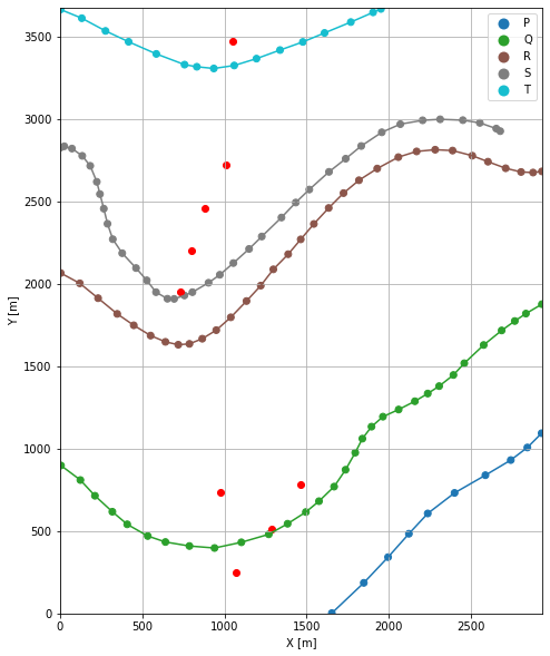
Plotting the Orientations#
[22]:
fig, ax = plt.subplots(1, figsize=(10, 10))

interfaces.plot(ax=ax, column='formation', legend=True, aspect='equal')
interfaces_coords.plot(ax=ax, column='formation', legend=True, aspect='equal')
orientations.plot(ax=ax, color='red', aspect='equal')
plt.grid()
ax.set_xlabel('X [m]')
ax.set_ylabel('Y [m]')
ax.set_xlim(0, 2932)
ax.set_ylim(0, 3677)
[22]:
(0.0, 3677.0)
GemPy Model Construction#
The structural geological model will be constructed using the GemPy package.
[23]:
import gempy as gp
WARNING (theano.configdefaults): g++ not available, if using conda: `conda install m2w64-toolchain`
WARNING (theano.configdefaults): g++ not detected ! Theano will be unable to execute optimized C-implementations (for both CPU and GPU) and will default to Python implementations. Performance will be severely degraded. To remove this warning, set Theano flags cxx to an empty string.
WARNING (theano.tensor.blas): Using NumPy C-API based implementation for BLAS functions.
Creating new Model#
[24]:
geo_model = gp.create_model('Model2')
geo_model
[24]:
Model2 2022-04-03 21:47
Initiate Data#
[25]:
gp.init_data(geo_model, [0, 2932, 0, 3677, -700, 1000], [100, 100, 100],
             surface_points_df=interfaces_coords,
             orientations_df=orientations,
             default_values=True)
Active grids: ['regular']
[25]:
Model2 2022-04-03 21:47
Model Surfaces#
[26]:
geo_model.surfaces
[26]:
| surface | series | order_surfaces | color | id | |
|---|---|---|---|---|---|
| 0 | P | Default series | 1 | #015482 | 1 |
| 1 | Q | Default series | 2 | #9f0052 | 2 |
| 2 | R | Default series | 3 | #ffbe00 | 3 |
| 3 | S | Default series | 4 | #728f02 | 4 |
| 4 | T | Default series | 5 | #443988 | 5 |
Mapping the Stack to Surfaces#
[27]:
gp.map_stack_to_surfaces(geo_model,
                         {'Strata': ('P', 'Q', 'R', 'S', 'T')},
                         remove_unused_series=True)
geo_model.add_surfaces('U')
[27]:
| surface | series | order_surfaces | color | id | |
|---|---|---|---|---|---|
| 0 | P | Strata | 1 | #015482 | 1 |
| 1 | Q | Strata | 2 | #9f0052 | 2 |
| 2 | R | Strata | 3 | #ffbe00 | 3 |
| 3 | S | Strata | 4 | #728f02 | 4 |
| 4 | T | Strata | 5 | #443988 | 5 |
| 5 | U | Strata | 6 | #ff3f20 | 6 |
Showing the Number of Data Points#
[28]:
gg.utils.show_number_of_data_points(geo_model=geo_model)
[28]:
| surface | series | order_surfaces | color | id | No. of Interfaces | No. of Orientations | |
|---|---|---|---|---|---|---|---|
| 0 | P | Strata | 1 | #015482 | 1 | 10 | 3 |
| 1 | Q | Strata | 2 | #9f0052 | 2 | 31 | 1 |
| 2 | R | Strata | 3 | #ffbe00 | 3 | 32 | 1 |
| 3 | S | Strata | 4 | #728f02 | 4 | 37 | 3 |
| 4 | T | Strata | 5 | #443988 | 5 | 16 | 1 |
| 5 | U | Strata | 6 | #ff3f20 | 6 | 0 | 0 |
Loading Digital Elevation Model#
[29]:
geo_model.set_topography(source='gdal', filepath=file_path + 'raster2.tif')
Cropped raster to geo_model.grid.extent.
depending on the size of the raster, this can take a while...
storing converted file...
Active grids: ['regular' 'topography']
[29]:
Grid Object. Values:
array([[  14.66      ,   18.385     , -691.5       ],
       [  14.66      ,   18.385     , -674.5       ],
       [  14.66      ,   18.385     , -657.5       ],
       ...,
       [2926.99658703, 3652.02038043,  629.80548096],
       [2926.99658703, 3662.01222826,  629.07196045],
       [2926.99658703, 3672.00407609,  628.35705566]])
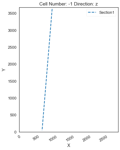
Defining Custom Section#
[30]:
custom_section = gpd.read_file(file_path + 'customsection2.shp')
custom_section_dict = gg.utils.to_section_dict(custom_section, section_column='name')
geo_model.set_section_grid(custom_section_dict)
Active grids: ['regular' 'topography' 'sections']
[30]:
| start | stop | resolution | dist | |
|---|---|---|---|---|
| Section1 | [974.6659586819704, 3627.5193764495925] | [676.0649712912196, 38.845314576599776] | [100, 80] | 3601.08 |
[31]:
gp.plot.plot_section_traces(geo_model)
[31]:
<gempy.plot.visualization_2d.Plot2D at 0x1c7084f8250>
Plotting Input Data#
[32]:
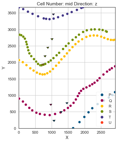
gp.plot_2d(geo_model, direction='z', show_lith=False, show_boundaries=False)
plt.grid()
[33]:
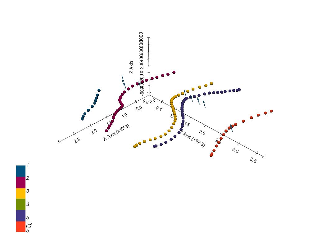
gp.plot_3d(geo_model, image=False, plotter_type='basic', notebook=True)
[33]:
<gempy.plot.vista.GemPyToVista at 0x1c706daf3d0>
Setting the Interpolator#
[34]:
gp.set_interpolator(geo_model,
                    compile_theano=True,
                    theano_optimizer='fast_compile',
                    verbose=[],
                    update_kriging=False
                    )
Compiling theano function...
Level of Optimization:  fast_compile
Device:  cpu
Precision:  float64
Number of faults:  0
Compilation Done!
Kriging values:
                    values
range              5000.7
$C_o$           595403.64
drift equations       [3]
[34]:
<gempy.core.interpolator.InterpolatorModel at 0x1c705297ee0>
Computing Model#
[35]:
sol = gp.compute_model(geo_model, compute_mesh=True)
Plotting Cross Sections#
[36]:
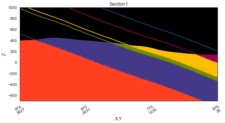
gp.plot_2d(geo_model, section_names=['Section1'], show_topography=True, show_data=False)
[36]:
<gempy.plot.visualization_2d.Plot2D at 0x1c709a2f430>
[37]:
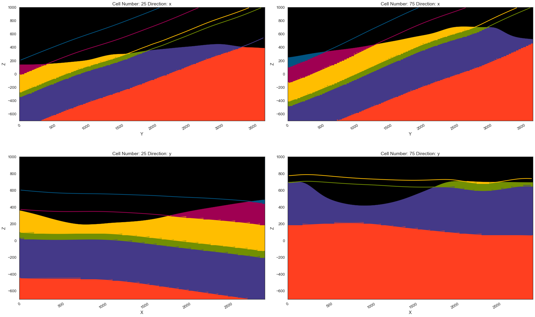
gp.plot_2d(geo_model, direction=['x', 'x', 'y', 'y'], cell_number=[25, 75, 25, 75], show_topography=True, show_data=False)
[37]:
<gempy.plot.visualization_2d.Plot2D at 0x1c709a2f5b0>
Plotting 3D Model#
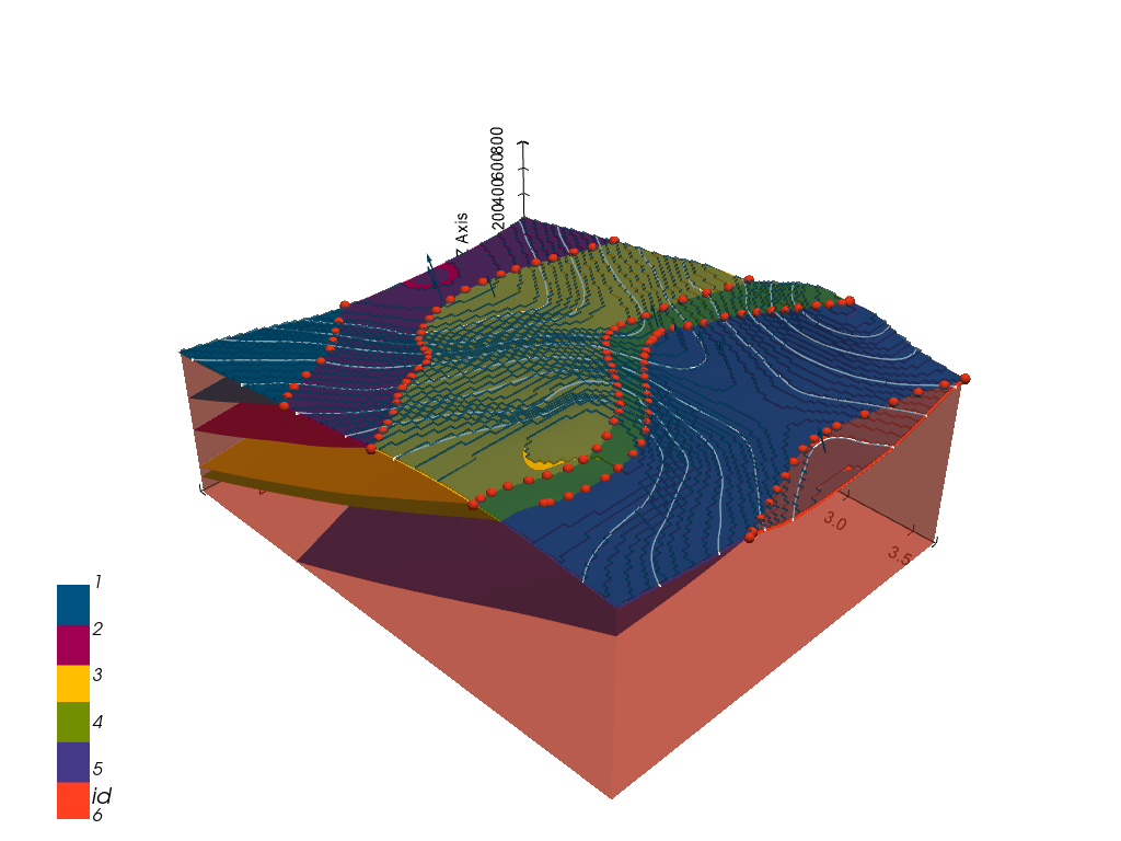
[38]:
gpv = gp.plot_3d(geo_model, image=False, show_topography=True,
                 plotter_type='basic', notebook=True, show_lith=True)
[ ]: