
Example 11 - Horizontal Layers
Contents
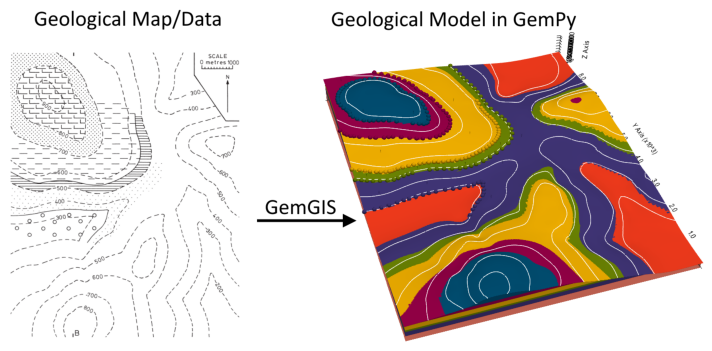
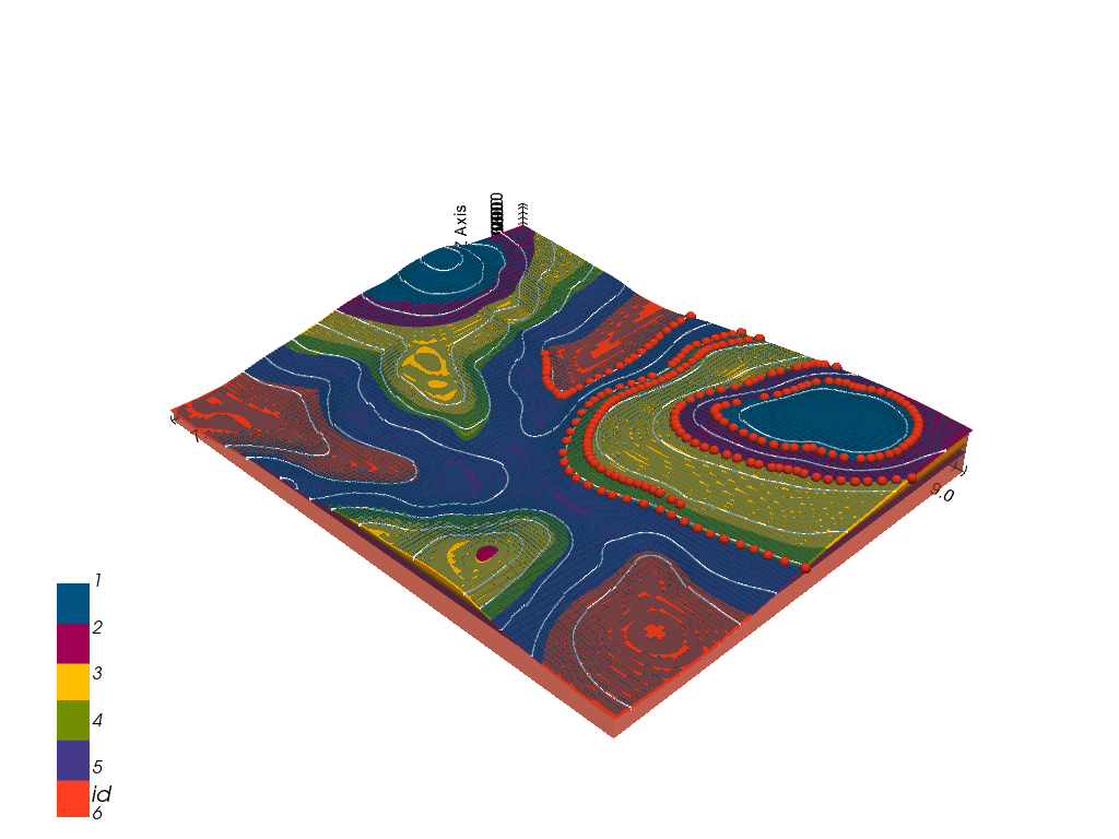
Example 11 - Horizontal Layers#
This example will show how to convert the geological map below using GemGIS to a GemPy model. This example is based on digitized data. The area is 7364 m wide (W-E extent) and 9176 m high (N-S extent). The vertical model extent varies between 0 m and 1000 m. The model represents horizontally deposited layers (blue to purple) above a basement (red). The map has been georeferenced with QGIS. The stratigraphic boundaries were digitized in QGIS. Strikes lines were digitized in QGIS as well
and will be used to calculate orientations for the GemPy model. The contour lines were also digitized and will be interpolated with GemGIS to create a topography for the model.
Map Source: An Introduction to Geological Structures and Maps by G.M. Bennison
[1]:
import matplotlib.pyplot as plt
import matplotlib.image as mpimg
img = mpimg.imread('../images/cover_example11.png')
plt.figure(figsize=(10, 10))
imgplot = plt.imshow(img)
plt.axis('off')
plt.tight_layout()
Licensing#
Computational Geosciences and Reservoir Engineering, RWTH Aachen University, Authors: Alexander Juestel. For more information contact: alexander.juestel(at)rwth-aachen.de
This work is licensed under a Creative Commons Attribution 4.0 International License (http://creativecommons.org/licenses/by/4.0/)
Import GemGIS#
If you have installed GemGIS via pip or conda, you can import GemGIS like any other package. If you have downloaded the repository, append the path to the directory where the GemGIS repository is stored and then import GemGIS.
[2]:
import warnings
warnings.filterwarnings("ignore")
import gemgis as gg
Importing Libraries and loading Data#
All remaining packages can be loaded in order to prepare the data and to construct the model. The example data is downloaded from an external server using pooch. It will be stored in a data folder in the same directory where this notebook is stored.
[3]:
import geopandas as gpd
import rasterio
[4]:
file_path = 'data/example11/'
gg.download_gemgis_data.download_tutorial_data(filename="example11_horizontal_layers.zip", dirpath=file_path)
Downloading file 'example11_horizontal_layers.zip' from 'https://rwth-aachen.sciebo.de/s/AfXRsZywYDbUF34/download?path=%2Fexample11_horizontal_layers.zip' to 'C:\Users\ale93371\Documents\gemgis\docs\getting_started\example\data\example11'.
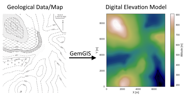
Creating Digital Elevation Model from Contour Lines#
The digital elevation model (DEM) will be created by interpolating contour lines digitized from the georeferenced map using the SciPy Radial Basis Function interpolation wrapped in GemGIS. The respective function used for that is gg.vector.interpolate_raster().
[5]:
import matplotlib.pyplot as plt
import matplotlib.image as mpimg
img = mpimg.imread('../images/dem_example11.png')
plt.figure(figsize=(10, 10))
imgplot = plt.imshow(img)
plt.axis('off')
plt.tight_layout()
[6]:
topo = gpd.read_file(file_path + 'topo11.shp')
topo.head()
[6]:
| id | Z | geometry | |
|---|---|---|---|
| 0 | None | 300 | LINESTRING (5554.550 9169.979, 5469.438 8954.3... |
| 1 | None | 400 | LINESTRING (4595.623 9164.305, 4696.339 8940.1... |
| 2 | None | 700 | LINESTRING (6411.342 6429.379, 6524.824 6460.5... |
| 3 | None | 600 | LINESTRING (7360.338 6813.800, 7170.255 6803.8... |
| 4 | None | 500 | LINESTRING (6784.415 7146.446, 6510.639 7045.7... |
Interpolating the contour lines#
[7]:
topo_raster = gg.vector.interpolate_raster(gdf=topo, value='Z', method='rbf', res=15)
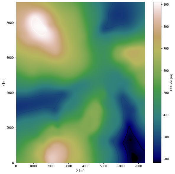
Plotting the raster#
[8]:
import matplotlib.pyplot as plt

fix, ax = plt.subplots(1, figsize=(10, 10))
topo.plot(ax=ax, aspect='equal', column='Z', cmap='gist_earth')
im = plt.imshow(topo_raster, origin='lower', extent=[0, 7364, 0, 9176], cmap='gist_earth')
cbar = plt.colorbar(im)
cbar.set_label('Altitude [m]')
ax.set_xlabel('X [m]')
ax.set_ylabel('Y [m]')
ax.set_xlim(0, 7364)
ax.set_ylim(0, 9176)
[8]:
(0.0, 9176.0)
Saving the raster to disc#
After the interpolation of the contour lines, the raster is saved to disc using gg.raster.save_as_tiff(). The function will not be executed as a raster is already provided with the example data.
Opening Raster#
The previously computed and saved raster can now be opened using rasterio.
[9]:
topo_raster = rasterio.open(file_path + 'raster11.tif')
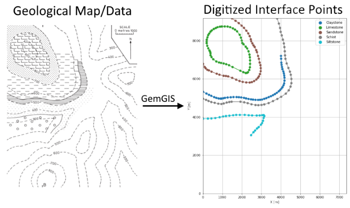
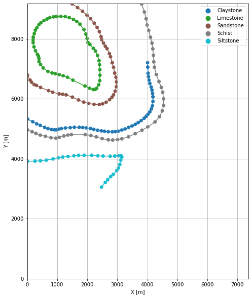
Interface Points of stratigraphic boundaries#
The interface points will be extracted from LineStrings digitized from the georeferenced map using QGIS. It is important to provide a formation name for each layer boundary. The vertical position of the interface point will be extracted from the digital elevation model using the GemGIS function gg.vector.extract_xyz(). The resulting GeoDataFrame now contains single points including the information about the respective formation.
[10]:
import matplotlib.pyplot as plt
import matplotlib.image as mpimg
img = mpimg.imread('../images/interfaces_example11.png')
plt.figure(figsize=(10, 10))
imgplot = plt.imshow(img)
plt.axis('off')
plt.tight_layout()
[11]:
interfaces = gpd.read_file(file_path + 'interfaces11.shp')
interfaces.head()
[11]:
| id | formation | geometry | |
|---|---|---|---|
| 0 | None | Limestone | LINESTRING (993.266 8745.838, 1122.353 8748.67... |
| 1 | None | Sandstone | LINESTRING (1496.845 9169.979, 1676.998 9043.7... |
| 2 | None | Claystone | LINESTRING (4006.933 7206.733, 4012.608 7058.4... |
| 3 | None | Schist | LINESTRING (3809.049 9166.432, 3899.834 8898.3... |
| 4 | None | Siltstone | LINESTRING (8.807 3915.744, 258.468 3921.418, ... |
Extracting Z coordinate from Digital Elevation Model#
[12]:
interfaces_coords = gg.vector.extract_xyz(gdf=interfaces, dem=topo_raster)
interfaces_coords = interfaces_coords[interfaces_coords['formation'].isin(['Limestone', 'Sandstone', 'Claystone', 'Schist', 'Siltstone'])]
interfaces_coords
[12]:
| formation | geometry | X | Y | Z | |
|---|---|---|---|---|---|
| 0 | Limestone | POINT (993.266 8745.838) | 993.27 | 8745.84 | 800.72 |
| 1 | Limestone | POINT (1122.353 8748.675) | 1122.35 | 8748.68 | 801.43 |
| 2 | Limestone | POINT (1267.043 8743.001) | 1267.04 | 8743.00 | 800.10 |
| 3 | Limestone | POINT (1398.966 8710.375) | 1398.97 | 8710.37 | 802.97 |
| 4 | Limestone | POINT (1539.401 8647.960) | 1539.40 | 8647.96 | 802.86 |
| ... | ... | ... | ... | ... | ... |
| 215 | Siltstone | POINT (2861.471 3478.836) | 2861.47 | 3478.84 | 364.48 |
| 216 | Siltstone | POINT (2776.359 3405.073) | 2776.36 | 3405.07 | 363.79 |
| 217 | Siltstone | POINT (2677.062 3300.101) | 2677.06 | 3300.10 | 357.72 |
| 218 | Siltstone | POINT (2596.205 3209.316) | 2596.21 | 3209.32 | 351.91 |
| 219 | Siltstone | POINT (2472.793 3054.696) | 2472.79 | 3054.70 | 338.67 |
220 rows × 5 columns
Plotting the Interface Points#
[13]:
fig, ax = plt.subplots(1, figsize=(10, 10))

interfaces.plot(ax=ax, column='formation', legend=True, aspect='equal')
interfaces_coords.plot(ax=ax, column='formation', legend=True, aspect='equal')
plt.grid()
ax.set_xlabel('X [m]')
ax.set_ylabel('Y [m]')
ax.set_xlim(0, 7364)
ax.set_ylim(0, 9176)
[13]:
(0.0, 9176.0)
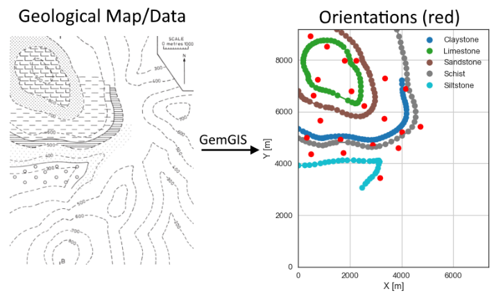
Orientations from Strike Lines#
Strike lines connect outcropping stratigraphic boundaries (interfaces) of the same altitude. In other words: the intersections between topographic contours and stratigraphic boundaries at the surface. The height difference and the horizontal difference between two digitized lines is used to calculate the dip and azimuth and hence an orientation that is necessary for GemPy. In order to calculate the orientations, each set of strikes lines/LineStrings for one formation must be given an id
number next to the altitude of the strike line. The id field is already predefined in QGIS. The strike line with the lowest altitude gets the id number 1, the strike line with the highest altitude the the number according to the number of digitized strike lines. It is currently recommended to use one set of strike lines for each structural element of one formation as illustrated.
For this example, the orientations were defined by points in QGIS as the layers were deposited horizontally and have no dip.
[14]:
import matplotlib.pyplot as plt
import matplotlib.image as mpimg
img = mpimg.imread('../images/orientations_example11.png')
plt.figure(figsize=(10, 10))
imgplot = plt.imshow(img)
plt.axis('off')
plt.tight_layout()
[15]:
orientations = gpd.read_file(file_path + 'orientations11.shp')
orientations = gg.vector.extract_xyz(gdf=orientations, dem=topo_raster)
orientations.head()
[15]:
| dip | azimuth | polarity | formation | geometry | X | Y | Z | |
|---|---|---|---|---|---|---|---|---|
| 0 | 0.00 | 0.00 | 1.00 | Limestone | POINT (1111.004 8516.036) | 1111.00 | 8516.04 | 867.24 |
| 1 | 0.00 | 0.00 | 1.00 | Limestone | POINT (2041.560 6791.104) | 2041.56 | 6791.10 | 842.33 |
| 2 | 0.00 | 0.00 | 1.00 | Limestone | POINT (747.861 7245.033) | 747.86 | 7245.03 | 837.07 |
| 3 | 0.00 | 0.00 | 1.00 | Limestone | POINT (1791.899 7971.321) | 1791.90 | 7971.32 | 848.08 |
| 4 | 0.00 | 0.00 | 1.00 | Sandstone | POINT (2540.883 6223.692) | 2540.88 | 6223.69 | 755.14 |
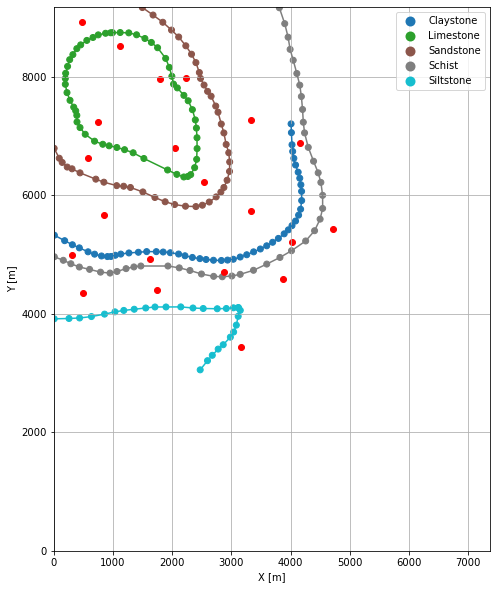
Plotting the Orientations#
[16]:
fig, ax = plt.subplots(1, figsize=(10, 10))

interfaces.plot(ax=ax, column='formation', legend=True, aspect='equal')
interfaces_coords.plot(ax=ax, column='formation', legend=True, aspect='equal')
orientations.plot(ax=ax, color='red', aspect='equal')
plt.grid()
plt.xlim(0,7364)
plt.ylim(0,9176)
plt.xlabel('X [m]')
plt.ylabel('Y [m]')
[16]:
Text(123.55887265135695, 0.5, 'Y [m]')
GemPy Model Construction#
The structural geological model will be constructed using the GemPy package.
[17]:
import gempy as gp
WARNING (theano.configdefaults): g++ not available, if using conda: `conda install m2w64-toolchain`
WARNING (theano.configdefaults): g++ not detected ! Theano will be unable to execute optimized C-implementations (for both CPU and GPU) and will default to Python implementations. Performance will be severely degraded. To remove this warning, set Theano flags cxx to an empty string.
WARNING (theano.tensor.blas): Using NumPy C-API based implementation for BLAS functions.
Creating new Model#
[18]:
geo_model = gp.create_model('Model11')
geo_model
[18]:
Model11 2022-04-05 11:02
Initiate Data#
[19]:
gp.init_data(geo_model, [0, 7364, 0, 9176, 0, 1000], [100, 100, 100],
             surface_points_df=interfaces_coords[interfaces_coords['Z'] != 0],
             orientations_df=orientations,
             default_values=True)
Active grids: ['regular']
[19]:
Model11 2022-04-05 11:02
Model Surfaces#
[20]:
geo_model.surfaces
[20]:
| surface | series | order_surfaces | color | id | |
|---|---|---|---|---|---|
| 0 | Limestone | Default series | 1 | #015482 | 1 |
| 1 | Sandstone | Default series | 2 | #9f0052 | 2 |
| 2 | Claystone | Default series | 3 | #ffbe00 | 3 |
| 3 | Schist | Default series | 4 | #728f02 | 4 |
| 4 | Siltstone | Default series | 5 | #443988 | 5 |
Mapping the Stack to Surfaces#
[21]:
gp.map_stack_to_surfaces(geo_model,
                         {
                          'Strata1': ('Limestone', 'Sandstone', 'Claystone', 'Schist', 'Siltstone'),
                         },
                         remove_unused_series=True)
geo_model.add_surfaces('Basement')
[21]:
| surface | series | order_surfaces | color | id | |
|---|---|---|---|---|---|
| 0 | Limestone | Strata1 | 1 | #015482 | 1 |
| 1 | Sandstone | Strata1 | 2 | #9f0052 | 2 |
| 2 | Claystone | Strata1 | 3 | #ffbe00 | 3 |
| 3 | Schist | Strata1 | 4 | #728f02 | 4 |
| 4 | Siltstone | Strata1 | 5 | #443988 | 5 |
| 5 | Basement | Strata1 | 6 | #ff3f20 | 6 |
Showing the Number of Data Points#
[22]:
gg.utils.show_number_of_data_points(geo_model=geo_model)
[22]:
| surface | series | order_surfaces | color | id | No. of Interfaces | No. of Orientations | |
|---|---|---|---|---|---|---|---|
| 0 | Limestone | Strata1 | 1 | #015482 | 1 | 54 | 4 |
| 1 | Sandstone | Strata1 | 2 | #9f0052 | 2 | 44 | 4 |
| 2 | Claystone | Strata1 | 3 | #ffbe00 | 3 | 50 | 3 |
| 3 | Schist | Strata1 | 4 | #728f02 | 4 | 43 | 5 |
| 4 | Siltstone | Strata1 | 5 | #443988 | 5 | 29 | 5 |
| 5 | Basement | Strata1 | 6 | #ff3f20 | 6 | 0 | 0 |
Loading Digital Elevation Model#
[23]:
geo_model.set_topography(
    source='gdal', filepath=file_path + 'raster11.tif')
Cropped raster to geo_model.grid.extent.
depending on the size of the raster, this can take a while...
storing converted file...
Active grids: ['regular' 'topography']
[23]:
Grid Object. Values:
array([[3.68200000e+01, 4.58800000e+01, 5.00000000e+00],
       [3.68200000e+01, 4.58800000e+01, 1.50000000e+01],
       [3.68200000e+01, 4.58800000e+01, 2.50000000e+01],
       ...,
       [7.35650102e+03, 9.13851634e+03, 3.66282013e+02],
       [7.35650102e+03, 9.15350980e+03, 3.66405060e+02],
       [7.35650102e+03, 9.16850327e+03, 3.66539032e+02]])
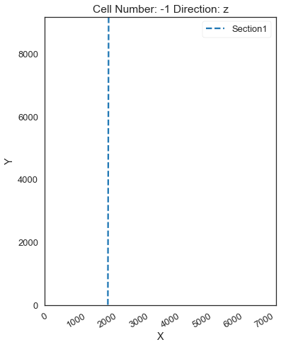
Defining Custom Section#
[24]:
custom_section = gpd.read_file(file_path + 'customsection11.shp')
custom_section_dict = gg.utils.to_section_dict(custom_section, section_column='name')
geo_model.set_section_grid(custom_section_dict)
Active grids: ['regular' 'topography' 'sections']
[24]:
| start | stop | resolution | dist | |
|---|---|---|---|---|
| Section1 | [2033.048983708095, 9169.978630835749] | [2008.9339736694492, 4.856286148714844] | [100, 80] | 9165.15 |
[25]:
gp.plot.plot_section_traces(geo_model)
[25]:
<gempy.plot.visualization_2d.Plot2D at 0x1b5ae7f52e0>
Plotting Input Data#
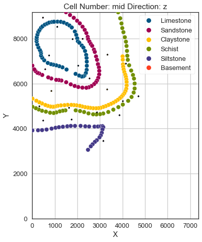
[26]:
gp.plot_2d(geo_model, direction='z', show_lith=False, show_boundaries=False)
plt.grid()
[27]:
gp.plot_3d(geo_model, image=False, plotter_type='basic', notebook=True)
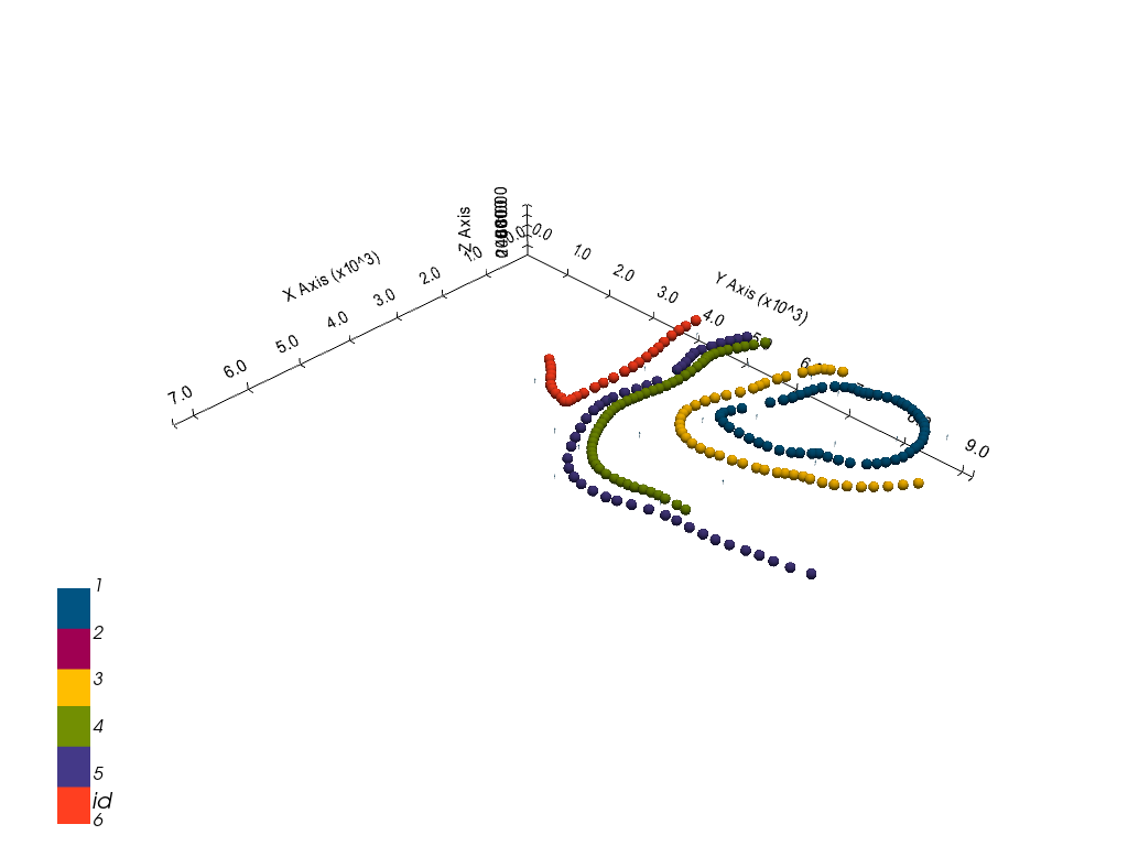
[27]:
<gempy.plot.vista.GemPyToVista at 0x1b5b036d3d0>
Setting the Interpolator#
[28]:
gp.set_interpolator(geo_model,
                    compile_theano=True,
                    theano_optimizer='fast_compile',
                    verbose=[],
                    update_kriging=False
                    )
Compiling theano function...
Level of Optimization:  fast_compile
Device:  cpu
Precision:  float64
Number of faults:  0
Compilation Done!
Kriging values:
                     values
range             11807.94
$C_o$           3319701.71
drift equations        [3]
[28]:
<gempy.core.interpolator.InterpolatorModel at 0x1b5ae7f5d90>
Computing Model#
[29]:
sol = gp.compute_model(geo_model, compute_mesh=True)
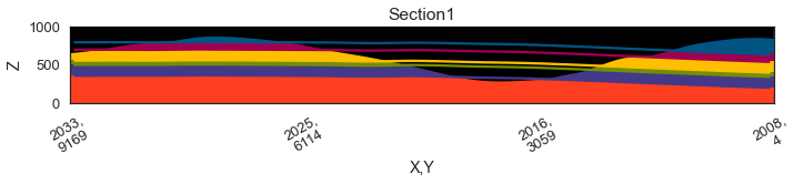
Plotting Cross Sections#
[30]:
gp.plot_2d(geo_model, section_names=['Section1'], show_topography=True, show_data=False)
[30]:
<gempy.plot.visualization_2d.Plot2D at 0x1b5b16055b0>
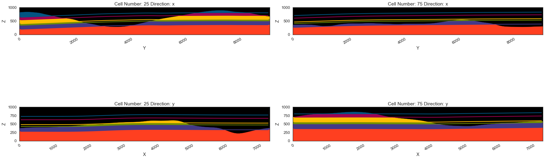
[31]:
gp.plot_2d(geo_model, direction=['x', 'x', 'y', 'y'], cell_number=[25, 75, 25, 75], show_topography=True, show_data=False)
[31]:
<gempy.plot.visualization_2d.Plot2D at 0x1b5b1a325b0>
Plotting 3D Model#
[32]:
gpv = gp.plot_3d(geo_model, image=False, show_topography=True,
                 plotter_type='basic', notebook=True, show_lith=True)
[ ]: