
Example 5 - Folded Layers
Contents
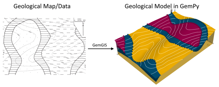
Example 5 - Folded Layers#
This example will show how to convert the geological map below using GemGIS to a GemPy model. This example is based on digitized data. The area is 3942 m wide (W-E extent) and 2710 m high (N-S extent). The vertical extent varies between -200 m and 1000 m. The model represents two folded layers (purple and blue) above a basement (yellow). The map has been georeferenced with QGIS. The stratigraphic boundaries were digitized in QGIS. Strikes lines were digitized in QGIS as well and will be
used to calculate orientations for the GemPy model. The contour lines were also digitized and will be interpolated with GemGIS to create a topography for the model.
Map Source: An Introduction to Geological Structures and Maps by G.M. Bennison
[1]:
import matplotlib.pyplot as plt
import matplotlib.image as mpimg
img = mpimg.imread('../images/cover_example05.png')
plt.figure(figsize=(10, 10))
imgplot = plt.imshow(img)
plt.axis('off')
plt.tight_layout()
Licensing#
Computational Geosciences and Reservoir Engineering, RWTH Aachen University, Authors: Alexander Juestel. For more information contact: alexander.juestel(at)rwth-aachen.de
This work is licensed under a Creative Commons Attribution 4.0 International License (http://creativecommons.org/licenses/by/4.0/)
Import GemGIS#
If you have installed GemGIS via pip or conda, you can import GemGIS like any other package. If you have downloaded the repository, append the path to the directory where the GemGIS repository is stored and then import GemGIS.
[2]:
import warnings
warnings.filterwarnings("ignore")
import gemgis as gg
Importing Libraries and loading Data#
All remaining packages can be loaded in order to prepare the data and to construct the model. The example data is downloaded from an external server using pooch. It will be stored in a data folder in the same directory where this notebook is stored.
[3]:
import geopandas as gpd
import rasterio
[4]:
file_path = 'data/example05/'
gg.download_gemgis_data.download_tutorial_data(filename="example05_folded_layers.zip", dirpath=file_path)
Downloading file 'example05_folded_layers.zip' from 'https://rwth-aachen.sciebo.de/s/AfXRsZywYDbUF34/download?path=%2Fexample05_folded_layers.zip' to 'C:\Users\ale93371\Documents\gemgis\docs\getting_started\example\data\example05'.
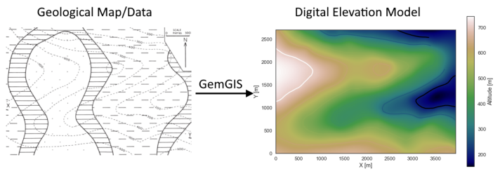
Creating Digital Elevation Model from Contour Lines#
The digital elevation model (DEM) will be created by interpolating contour lines digitized from the georeferenced map using the SciPy Radial Basis Function interpolation wrapped in GemGIS. The respective function used for that is gg.vector.interpolate_raster().
[5]:
import matplotlib.pyplot as plt
import matplotlib.image as mpimg
img = mpimg.imread('../images/dem_example05.png')
plt.figure(figsize=(10, 10))
imgplot = plt.imshow(img)
plt.axis('off')
plt.tight_layout()
[6]:
topo = gpd.read_file(file_path + 'topo5.shp')
topo.head()
[6]:
| id | Z | geometry | |
|---|---|---|---|
| 0 | None | 700 | LINESTRING (1.537 2299.193, 29.191 2272.378, 7... |
| 1 | None | 600 | LINESTRING (81.145 2708.127, 130.586 2641.927,... |
| 2 | None | 600 | LINESTRING (6.565 403.682, 56.006 360.945, 103... |
| 3 | None | 600 | LINESTRING (3278.040 2.289, 3308.208 32.456, 3... |
| 4 | None | 600 | LINESTRING (2258.218 1964.001, 2375.536 1953.1... |
Interpolating the contour lines#
[7]:
topo_raster = gg.vector.interpolate_raster(gdf=topo, value='Z', method='rbf', res=10)
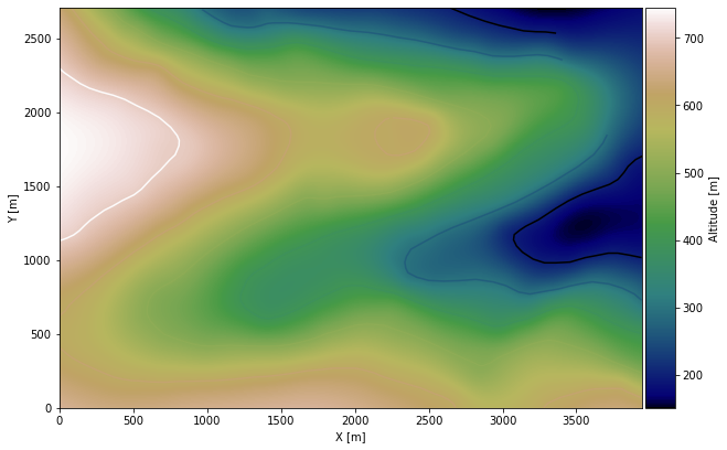
Plotting the raster#
[8]:
import matplotlib.pyplot as plt

from mpl_toolkits.axes_grid1 import make_axes_locatable
fix, ax = plt.subplots(1, figsize=(10, 10))
topo.plot(ax=ax, aspect='equal', column='Z', cmap='gist_earth')
im = plt.imshow(topo_raster, origin='lower', extent=[0, 3942, 0, 2710], cmap='gist_earth')
divider = make_axes_locatable(ax)
cax = divider.append_axes("right", size="5%", pad=0.05)
cbar = plt.colorbar(im, cax=cax)
cbar.set_label('Altitude [m]')
ax.set_xlabel('X [m]')
ax.set_ylabel('Y [m]')
ax.set_xlim(0, 3942)
ax.set_ylim(0, 2710)
[8]:
(0.0, 2710.0)
Saving the raster to disc#
After the interpolation of the contour lines, the raster is saved to disc using gg.raster.save_as_tiff(). The function will not be executed as a raster is already provided with the example data.
Opening Raster#
The previously computed and saved raster can now be opened using rasterio.
[9]:
topo_raster = rasterio.open(file_path + 'raster5.tif')
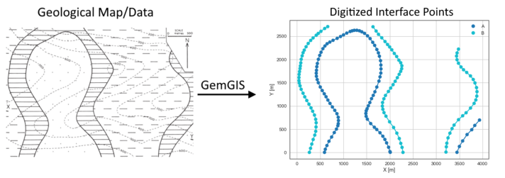
Interface Points of stratigraphic boundaries#
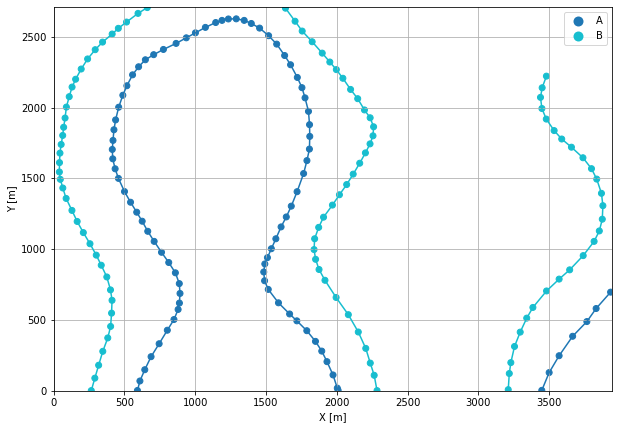
The interface points will be extracted from LineStrings digitized from the georeferenced map using QGIS. It is important to provide a formation name for each layer boundary. The vertical position of the interface point will be extracted from the digital elevation model using the GemGIS function gg.vector.extract_xyz(). The resulting GeoDataFrame now contains single points including the information about the respective formation.
[10]:
import matplotlib.pyplot as plt
import matplotlib.image as mpimg
img = mpimg.imread('../images/interfaces_example05.png')
plt.figure(figsize=(10, 10))
imgplot = plt.imshow(img)
plt.axis('off')
plt.tight_layout()
[11]:
interfaces = gpd.read_file(file_path + 'interfaces5.shp')
interfaces.head()
[11]:
| id | formation | geometry | |
|---|---|---|---|
| 0 | None | A | LINESTRING (591.475 2.289, 609.073 69.327, 643... |
| 1 | None | A | LINESTRING (3448.150 3.127, 3500.105 128.824, ... |
| 2 | None | B | LINESTRING (265.501 1.451, 290.641 89.439, 317... |
| 3 | None | B | LINESTRING (2284.196 1.451, 2264.084 109.550, ... |
| 4 | None | B | LINESTRING (3480.832 2222.937, 3450.664 2140.8... |
Extracting Z coordinate from Digital Elevation Model#
[12]:
interfaces_coords = gg.vector.extract_xyz(gdf=interfaces, dem=topo_raster)
interfaces_coords = interfaces_coords.sort_values(by='formation', ascending=False)
interfaces_coords
[12]:
| formation | geometry | X | Y | Z | |
|---|---|---|---|---|---|
| 94 | B | POINT (412.148 639.154) | 412.15 | 639.15 | 538.20 |
| 129 | B | POINT (2204.588 299.772) | 2204.59 | 299.77 | 578.98 |
| 120 | B | POINT (345.109 2463.437) | 345.11 | 2463.44 | 588.11 |
| 121 | B | POINT (412.986 2520.420) | 412.99 | 2520.42 | 547.54 |
| 122 | B | POINT (456.561 2560.643) | 456.56 | 2560.64 | 518.60 |
| ... | ... | ... | ... | ... | ... |
| 61 | A | POINT (1643.141 1228.254) | 1643.14 | 1228.25 | 436.22 |
| 62 | A | POINT (1606.270 1157.864) | 1606.27 | 1157.86 | 419.63 |
| 63 | A | POINT (1569.399 1074.066) | 1569.40 | 1074.07 | 402.09 |
| 64 | A | POINT (1537.555 1003.675) | 1537.56 | 1003.68 | 390.91 |
| 0 | A | POINT (591.475 2.289) | 591.48 | 2.29 | 641.21 |
188 rows × 5 columns
Plotting the Interface Points#
[13]:
fig, ax = plt.subplots(1, figsize=(10, 10))

interfaces.plot(ax=ax, column='formation', legend=True, aspect='equal')
interfaces_coords.plot(ax=ax, column='formation', legend=True, aspect='equal')
plt.grid()
ax.set_xlabel('X [m]')
ax.set_ylabel('Y [m]')
ax.set_xlim(0, 3942)
ax.set_ylim(0, 2710)
[13]:
(0.0, 2710.0)
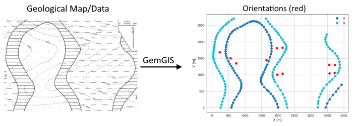
Orientations from Strike Lines#
Strike lines connect outcropping stratigraphic boundaries (interfaces) of the same altitude. In other words: the intersections between topographic contours and stratigraphic boundaries at the surface. The height difference and the horizontal difference between two digitized lines is used to calculate the dip and azimuth and hence an orientation that is necessary for GemPy. In order to calculate the orientations, each set of strikes lines/LineStrings for one formation must be given an id
number next to the altitude of the strike line. The id field is already predefined in QGIS. The strike line with the lowest altitude gets the id number 1, the strike line with the highest altitude the the number according to the number of digitized strike lines. It is currently recommended to use one set of strike lines for each structural element of one formation as illustrated.
[14]:
import matplotlib.pyplot as plt
import matplotlib.image as mpimg
img = mpimg.imread('../images/orientations_example05.png')
plt.figure(figsize=(10, 10))
imgplot = plt.imshow(img)
plt.axis('off')
plt.tight_layout()
[15]:
strikes = gpd.read_file(file_path + 'strikes5.shp')
strikes
[15]:
| id | formation | Z | geometry | |
|---|---|---|---|---|
| 0 | 2 | B1 | 700 | LINESTRING (149.860 2191.094, 154.888 1214.846) |
| 1 | 1 | B1 | 600 | LINESTRING (319.551 2436.622, 321.855 916.106) |
| 2 | 3 | A1 | 700 | LINESTRING (481.281 2067.910, 488.404 1433.140) |
| 3 | 2 | A1 | 600 | LINESTRING (636.098 2326.846, 655.529 174.023) |
| 4 | 1 | A1 | 500 | LINESTRING (807.413 2426.933, 822.287 456.422) |
| 5 | 2 | A2 | 500 | LINESTRING (1725.629 2204.030, 1737.885 473.391) |
| 6 | 1 | A2 | 400 | LINESTRING (1556.253 2469.041, 1567.356 648.529) |
| 7 | 1 | B2 | 400 | LINESTRING (1890.816 1193.007, 1900.453 810.050) |
| 8 | 2 | B2 | 500 | LINESTRING (2062.183 564.521, 2056.317 1437.278) |
| 9 | 3 | B2 | 600 | LINESTRING (2216.791 1955.150, 2236.483 196.648) |
| 10 | 2 | B3 | 500 | LINESTRING (2056.527 1437.278, 2055.479 2190.203) |
| 11 | 3 | B3 | 600 | LINESTRING (2216.581 1954.312, 2220.352 1718.839) |
| 12 | 1 | B3 | 400 | LINESTRING (1877.199 2407.659, 1890.816 1192.692) |
| 13 | 1 | B4 | 200 | LINESTRING (3799.212 1567.165, 3810.106 1043.427) |
| 14 | 2 | B4 | 300 | LINESTRING (3636.644 1737.275, 3642.509 847.340) |
| 15 | 3 | B4 | 400 | LINESTRING (3469.048 1945.932, 3469.886 688.961) |
| 16 | 3 | A | 600 | LINESTRING (3487.483 96.509, 3487.902 1969.395) |
| 17 | 2 | A | 500 | LINESTRING (3647.118 355.445, 3637.063 1740.627) |
| 18 | 1 | A | 400 | LINESTRING (3808.639 548.600, 3790.413 1580.992) |
Calculate Orientations for each formation#
[16]:
orientations_a = gg.vector.calculate_orientations_from_strike_lines(gdf=strikes[strikes['formation'] == 'A'].sort_values(by='Z', ascending=True).reset_index())
orientations_a
[16]:
| dip | azimuth | Z | geometry | polarity | formation | X | Y | |
|---|---|---|---|---|---|---|---|---|
| 0 | 33.31 | 89.37 | 450.00 | POINT (3720.808 1056.416) | 1.00 | A | 3720.81 | 1056.42 |
| 1 | 33.83 | 89.86 | 550.00 | POINT (3564.892 1040.494) | 1.00 | A | 3564.89 | 1040.49 |
[17]:
orientations_a1 = gg.vector.calculate_orientations_from_strike_lines(gdf=strikes[strikes['formation'] == 'A1'].sort_values(by='Z', ascending=True).reset_index())
orientations_a1
[17]:
| dip | azimuth | Z | geometry | polarity | formation | X | Y | |
|---|---|---|---|---|---|---|---|---|
| 0 | 30.57 | 89.52 | 550.00 | POINT (730.331 1346.056) | 1.00 | A1 | 730.33 | 1346.06 |
| 1 | 32.70 | 89.47 | 650.00 | POINT (565.328 1500.480) | 1.00 | A1 | 565.33 | 1500.48 |
[18]:
orientations_a2 = gg.vector.calculate_orientations_from_strike_lines(gdf=strikes[strikes['formation'] == 'A2'].sort_values(by='Z', ascending=True).reset_index())
orientations_a2
[18]:
| dip | azimuth | Z | geometry | polarity | formation | X | Y | |
|---|---|---|---|---|---|---|---|---|
| 0 | 30.80 | 269.62 | 450.00 | POINT (1646.781 1448.748) | 1.00 | A2 | 1646.78 | 1448.75 |
[19]:
orientations_b1 = gg.vector.calculate_orientations_from_strike_lines(gdf=strikes[strikes['formation'] == 'B1'].sort_values(by='Z', ascending=True).reset_index())
orientations_b1
[19]:
| dip | azimuth | Z | geometry | polarity | formation | X | Y | |
|---|---|---|---|---|---|---|---|---|
| 0 | 30.99 | 89.85 | 650.00 | POINT (236.538 1689.667) | 1.00 | B1 | 236.54 | 1689.67 |
[20]:
orientations_b2 = gg.vector.calculate_orientations_from_strike_lines(gdf=strikes[strikes['formation'] == 'B2'].sort_values(by='Z', ascending=True).reset_index())
orientations_b2
[20]:
| dip | azimuth | Z | geometry | polarity | formation | X | Y | |
|---|---|---|---|---|---|---|---|---|
| 0 | 31.99 | 269.44 | 450.00 | POINT (1977.443 1001.214) | 1.00 | B2 | 1977.44 | 1001.21 |
| 1 | 31.03 | 269.41 | 550.00 | POINT (2142.944 1038.399) | 1.00 | B2 | 2142.94 | 1038.40 |
[21]:
orientations_b3 = gg.vector.calculate_orientations_from_strike_lines(gdf=strikes[strikes['formation'] == 'B3'].sort_values(by='Z', ascending=True).reset_index())
orientations_b3
[21]:
| dip | azimuth | Z | geometry | polarity | formation | X | Y | |
|---|---|---|---|---|---|---|---|---|
| 0 | 30.70 | 269.51 | 450.00 | POINT (1970.005 1806.958) | 1.00 | B3 | 1970.01 | 1806.96 |
| 1 | 31.88 | 269.85 | 550.00 | POINT (2137.235 1825.158) | 1.00 | B3 | 2137.23 | 1825.16 |
[22]:
orientations_b4 = gg.vector.calculate_orientations_from_strike_lines(gdf=strikes[strikes['formation'] == 'B4'].sort_values(by='Z', ascending=True).reset_index())
orientations_b4
[22]:
| dip | azimuth | Z | geometry | polarity | formation | X | Y | |
|---|---|---|---|---|---|---|---|---|
| 0 | 31.77 | 89.41 | 250.00 | POINT (3722.118 1298.802) | 1.00 | B4 | 3722.12 | 1298.80 |
| 1 | 30.84 | 89.85 | 350.00 | POINT (3554.522 1304.877) | 1.00 | B4 | 3554.52 | 1304.88 |
Merging Orientations#
[23]:
import pandas as pd
orientations = pd.concat([orientations_a, orientations_a1, orientations_a2, orientations_b1, orientations_b2, orientations_b3, orientations_b4]).reset_index()
orientations['formation'] = ['A', 'A', 'A', 'A', 'A', 'B', 'B', 'B', 'B', 'B', 'B', 'B']
orientations
[23]:
| index | dip | azimuth | Z | geometry | polarity | formation | X | Y | |
|---|---|---|---|---|---|---|---|---|---|
| 0 | 0 | 33.31 | 89.37 | 450.00 | POINT (3720.808 1056.416) | 1.00 | A | 3720.81 | 1056.42 |
| 1 | 1 | 33.83 | 89.86 | 550.00 | POINT (3564.892 1040.494) | 1.00 | A | 3564.89 | 1040.49 |
| 2 | 0 | 30.57 | 89.52 | 550.00 | POINT (730.331 1346.056) | 1.00 | A | 730.33 | 1346.06 |
| 3 | 1 | 32.70 | 89.47 | 650.00 | POINT (565.328 1500.480) | 1.00 | A | 565.33 | 1500.48 |
| 4 | 0 | 30.80 | 269.62 | 450.00 | POINT (1646.781 1448.748) | 1.00 | A | 1646.78 | 1448.75 |
| 5 | 0 | 30.99 | 89.85 | 650.00 | POINT (236.538 1689.667) | 1.00 | B | 236.54 | 1689.67 |
| 6 | 0 | 31.99 | 269.44 | 450.00 | POINT (1977.443 1001.214) | 1.00 | B | 1977.44 | 1001.21 |
| 7 | 1 | 31.03 | 269.41 | 550.00 | POINT (2142.944 1038.399) | 1.00 | B | 2142.94 | 1038.40 |
| 8 | 0 | 30.70 | 269.51 | 450.00 | POINT (1970.005 1806.958) | 1.00 | B | 1970.01 | 1806.96 |
| 9 | 1 | 31.88 | 269.85 | 550.00 | POINT (2137.235 1825.158) | 1.00 | B | 2137.23 | 1825.16 |
| 10 | 0 | 31.77 | 89.41 | 250.00 | POINT (3722.118 1298.802) | 1.00 | B | 3722.12 | 1298.80 |
| 11 | 1 | 30.84 | 89.85 | 350.00 | POINT (3554.522 1304.877) | 1.00 | B | 3554.52 | 1304.88 |
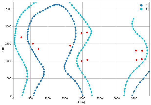
Plotting the Orientations#
[24]:
fig, ax = plt.subplots(1, figsize=(10, 10))

interfaces.plot(ax=ax, column='formation', legend=True, aspect='equal')
interfaces_coords.plot(ax=ax, column='formation', legend=True, aspect='equal')
orientations.plot(ax=ax, color='red', aspect='equal')
plt.grid()
ax.set_xlabel('X [m]')
ax.set_ylabel('Y [m]')
ax.set_xlim(0, 3942)
ax.set_ylim(0, 2710)
[24]:
(0.0, 2710.0)
GemPy Model Construction#
The structural geological model will be constructed using the GemPy package.
[25]:
import gempy as gp
WARNING (theano.configdefaults): g++ not available, if using conda: `conda install m2w64-toolchain`
WARNING (theano.configdefaults): g++ not detected ! Theano will be unable to execute optimized C-implementations (for both CPU and GPU) and will default to Python implementations. Performance will be severely degraded. To remove this warning, set Theano flags cxx to an empty string.
WARNING (theano.tensor.blas): Using NumPy C-API based implementation for BLAS functions.
Creating new Model#
[26]:
geo_model = gp.create_model('Model5')
geo_model
[26]:
Model5 2022-04-04 20:51
Initiate Data#
[27]:
gp.init_data(geo_model, [0, 3942, 0, 2710, -200, 1000], [100, 100, 100],
             surface_points_df=interfaces_coords[interfaces_coords['Z'] != 0],
             orientations_df=orientations,
             default_values=True)
Active grids: ['regular']
[27]:
Model5 2022-04-04 20:51
Model Surfaces#
[28]:
geo_model.surfaces
[28]:
| surface | series | order_surfaces | color | id | |
|---|---|---|---|---|---|
| 0 | B | Default series | 1 | #015482 | 1 |
| 1 | A | Default series | 2 | #9f0052 | 2 |
Mapping the Stack to Surfaces#
[29]:
gp.map_stack_to_surfaces(geo_model,
                         {
                          'Strata1': ('A', 'B'),
                         },
                         remove_unused_series=True)
geo_model.add_surfaces('Basement')
[29]:
| surface | series | order_surfaces | color | id | |
|---|---|---|---|---|---|
| 0 | B | Strata1 | 1 | #015482 | 1 |
| 1 | A | Strata1 | 2 | #9f0052 | 2 |
| 2 | Basement | Strata1 | 3 | #ffbe00 | 3 |
Showing the Number of Data Points#
[30]:
gg.utils.show_number_of_data_points(geo_model=geo_model)
[30]:
| surface | series | order_surfaces | color | id | No. of Interfaces | No. of Orientations | |
|---|---|---|---|---|---|---|---|
| 0 | B | Strata1 | 1 | #015482 | 1 | 101 | 7 |
| 1 | A | Strata1 | 2 | #9f0052 | 2 | 87 | 5 |
| 2 | Basement | Strata1 | 3 | #ffbe00 | 3 | 0 | 0 |
Loading Digital Elevation Model#
[31]:
geo_model.set_topography(
    source='gdal', filepath=file_path + 'raster5.tif')
Cropped raster to geo_model.grid.extent.
depending on the size of the raster, this can take a while...
storing converted file...
Active grids: ['regular' 'topography']
[31]:
Grid Object. Values:
array([[  19.71      ,   13.55      , -194.        ],
       [  19.71      ,   13.55      , -182.        ],
       [  19.71      ,   13.55      , -170.        ],
       ...,
       [3937.01012658, 2685.        ,  182.10906982],
       [3937.01012658, 2695.        ,  181.02072144],
       [3937.01012658, 2705.        ,  179.95965576]])
Defining Custom Section#
[32]:
custom_section = gpd.read_file(file_path + 'customsection5.shp')
custom_section_dict = gg.utils.to_section_dict(custom_section, section_column='name')
geo_model.set_section_grid(custom_section_dict)
Active grids: ['regular' 'topography' 'sections']
[32]:
| start | stop | resolution | dist | |
|---|---|---|---|---|
| Section1 | [6.565213969151387, 963.4523850507635] | [3931.665030709532, 366.8103975359992] | [100, 80] | 3970.19 |
[33]:
gp.plot.plot_section_traces(geo_model)
[33]:
<gempy.plot.visualization_2d.Plot2D at 0x2388552d640>
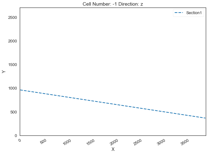
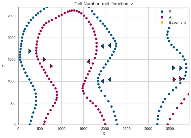
Plotting Input Data#
[34]:
gp.plot_2d(geo_model, direction='z', show_lith=False, show_boundaries=False)
plt.grid()
[35]:
gp.plot_3d(geo_model, image=False, plotter_type='basic', notebook=True)
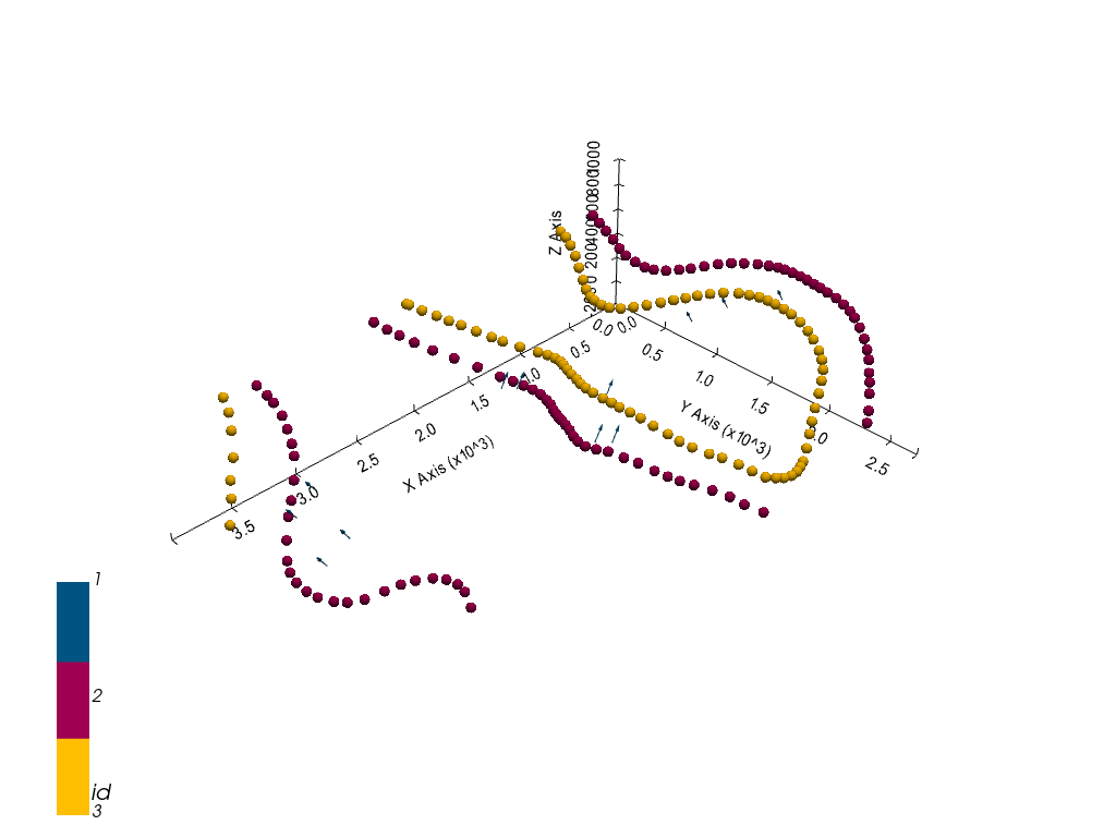
[35]:
<gempy.plot.vista.GemPyToVista at 0x238870ec850>
Setting the Interpolator#
[36]:
gp.set_interpolator(geo_model,
                    compile_theano=True,
                    theano_optimizer='fast_compile',
                    verbose=[],
                    update_kriging=False
                    )
Compiling theano function...
Level of Optimization:  fast_compile
Device:  cpu
Precision:  float64
Number of faults:  0
Compilation Done!
Kriging values:
                   values
range            4931.88
$C_o$           579130.1
drift equations      [3]
[36]:
<gempy.core.interpolator.InterpolatorModel at 0x238855398e0>
Computing Model#
[37]:
sol = gp.compute_model(geo_model, compute_mesh=True)
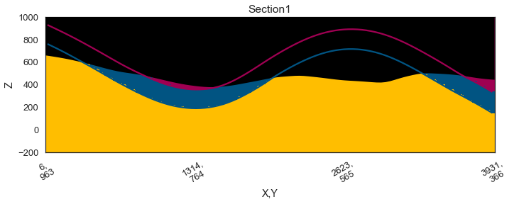
Plotting Cross Sections#
[38]:
gp.plot_2d(geo_model, section_names=['Section1'], show_topography=True, show_data=False)
[38]:
<gempy.plot.visualization_2d.Plot2D at 0x2388ccabf40>
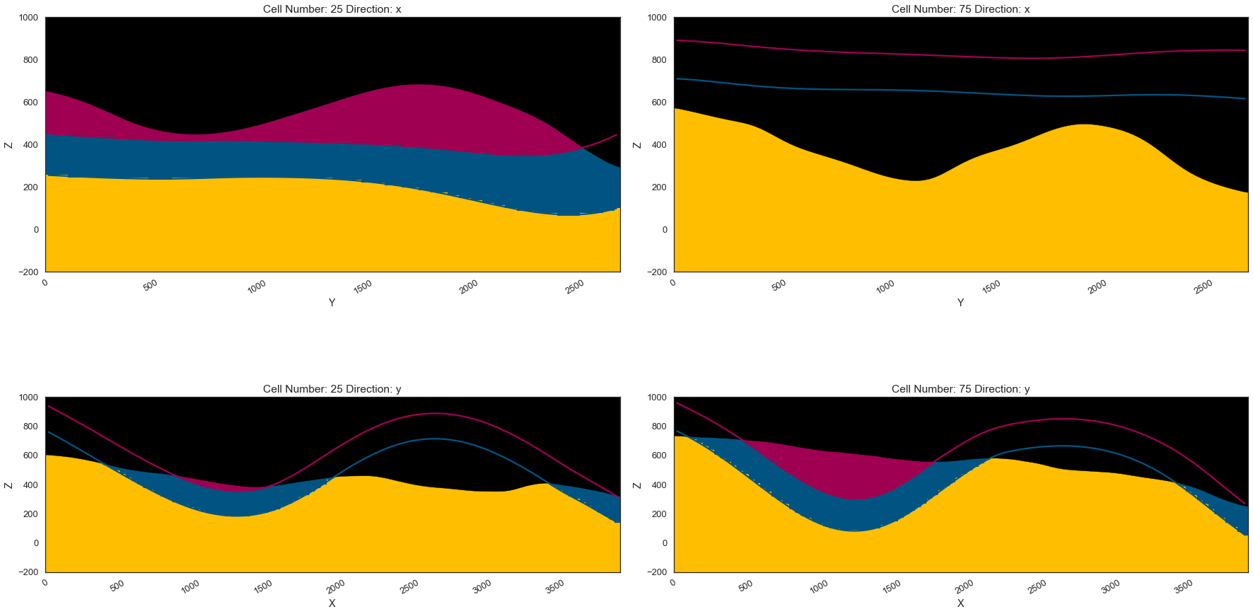
[39]:
gp.plot_2d(geo_model, direction=['x', 'x', 'y', 'y'], cell_number=[25, 75, 25, 75], show_topography=True, show_data=False)
[39]:
<gempy.plot.visualization_2d.Plot2D at 0x2388cff4ee0>
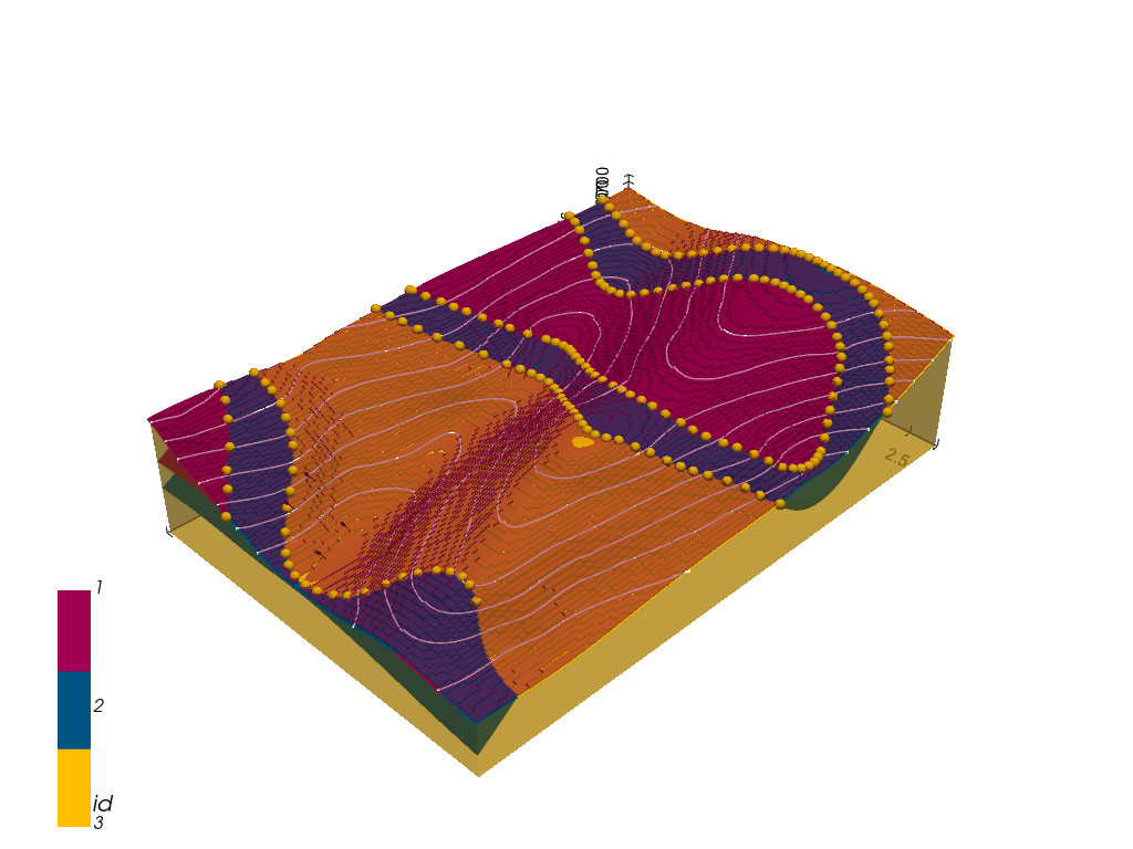
Plotting 3D Model#
[40]:
gpv = gp.plot_3d(geo_model, image=False, show_topography=True,
                 plotter_type='basic', notebook=True, show_lith=True)
[ ]: