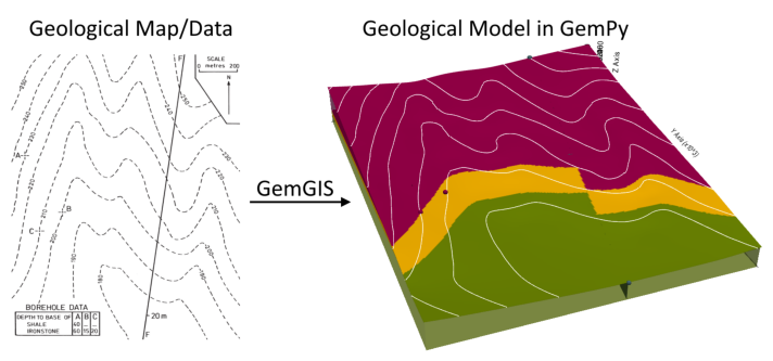
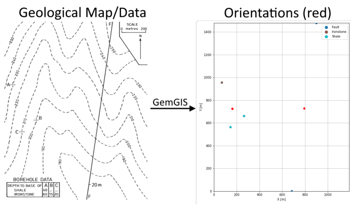
Example 15 - Three Point Problem#

This example will show how to convert the geological map below using GemGIS to a GemPy model. This example is based on digitized data. The area is 1187 m wide (W-E extent) and 1479 m high (N-S extent). The vertical model extent varies between 100 m and 300 m. This example represents a classic “three-point-problem” of planar dipping layers (green and yellow) above an unspecified basement (purple) which are separated by a fault (blue). The interface points were not recorded at the surface but rather in boreholes at depth. The fault has an offset of 20 m but no further interface points are located beyond the fault. This will be dealt with in a two model approach.

The map has been georeferenced with QGIS. The outcrops of the layers were digitized in QGIS. The contour lines were also digitized and will be interpolated with GemGIS to create a topography for the model.

Map Source: An Introduction to Geological Structures and Maps by G.M. Bennison

[1]:

import matplotlib.pyplot as plt
import matplotlib.image as mpimg
img = mpimg.imread('../images/cover_example15.png')
plt.figure(figsize=(10, 10))
imgplot = plt.imshow(img)
plt.axis('off')
plt.tight_layout()

../../_images/getting_started_example_example15_2_0.png

Licensing#

Computational Geosciences and Reservoir Engineering, RWTH Aachen University, Authors: Alexander Juestel. For more information contact: alexander.juestel(at)rwth-aachen.de

This work is licensed under a Creative Commons Attribution 4.0 International License (http://creativecommons.org/licenses/by/4.0/)

Import GemGIS#

If you have installed GemGIS via pip or conda, you can import GemGIS like any other package. If you have downloaded the repository, append the path to the directory where the GemGIS repository is stored and then import GemGIS.

[2]:

import warnings
warnings.filterwarnings("ignore")
import gemgis as gg

Importing Libraries and loading Data#

All remaining packages can be loaded in order to prepare the data and to construct the model. The example data is downloaded from an external server using pooch. It will be stored in a data folder in the same directory where this notebook is stored.

[3]:

import geopandas as gpd
import rasterio

[4]:

file_path = 'data/example15/'
gg.download_gemgis_data.download_tutorial_data(filename="example15_three_point_problem.zip", dirpath=file_path)

Downloading file 'example15_three_point_problem.zip' from 'https://rwth-aachen.sciebo.de/s/AfXRsZywYDbUF34/download?path=%2Fexample15_three_point_problem.zip' to 'C:\Users\ale93371\Documents\gemgis\docs\getting_started\example\data\example15'.

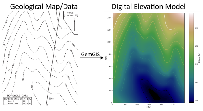
Creating Digital Elevation Model from Contour Lines#

The digital elevation model (DEM) will be created by interpolating contour lines digitized from the georeferenced map using the SciPy Radial Basis Function interpolation wrapped in GemGIS. The respective function used for that is gg.vector.interpolate_raster().

[5]:

import matplotlib.pyplot as plt
import matplotlib.image as mpimg
img = mpimg.imread('../images/dem_example15.png')
plt.figure(figsize=(10, 10))
imgplot = plt.imshow(img)
plt.axis('off')
plt.tight_layout()

../../_images/getting_started_example_example15_10_0.png

[6]:

topo = gpd.read_file(file_path + 'topo15.shp')
topo.head()

[6]:

	id	Z	geometry
0	None	180	LINESTRING (608.177 -0.021, 598.911 22.516, 58...
1	None	190	LINESTRING (323.662 216.425, 321.832 254.178, ...
2	None	200	LINESTRING (142.794 190.113, 153.433 227.980, ...
3	None	250	LINESTRING (1.395 1193.695, 20.385 1232.592, 3...
4	None	240	LINESTRING (1.623 925.311, 8.487 939.039, 13.7...

Interpolating the contour lines#

[7]:

topo_raster = gg.vector.interpolate_raster(gdf=topo, value='Z', method='rbf', res=5)

Plotting the raster#

[8]:

import matplotlib.pyplot as plt

fix, ax = plt.subplots(1, figsize=(10, 10))
topo.plot(ax=ax, aspect='equal', column='Z', cmap='gist_earth')
im = plt.imshow(topo_raster, origin='lower', extent=[0, 1187, 0, 1479], cmap='gist_earth')
cbar = plt.colorbar(im)
cbar.set_label('Altitude [m]')
ax.set_xlabel('X [m]')
ax.set_ylabel('Y [m]')
ax.set_xlim(0, 1187)
ax.set_ylim(0, 1479)

[8]:

(0.0, 1479.0)

../../_images/getting_started_example_example15_15_1.png

Saving the raster to disc#

After the interpolation of the contour lines, the raster is saved to disc using gg.raster.save_as_tiff(). The function will not be executed as a raster is already provided with the example data.

gg.raster.save_as_tiff(raster=topo_raster, path=file_path + 'raster15.tif', extent=[0, 1187, 0, 1479], crs='EPSG:4326', overwrite_file=True)

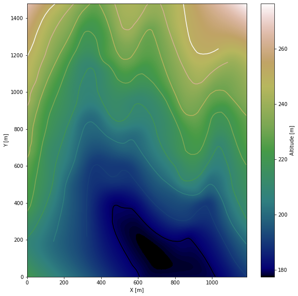
Opening Raster#

The previously computed and saved raster can now be opened using rasterio.

[9]:

topo_raster = rasterio.open(file_path + 'raster15.tif')

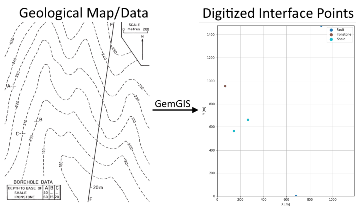
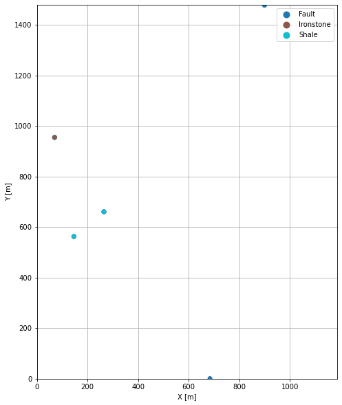
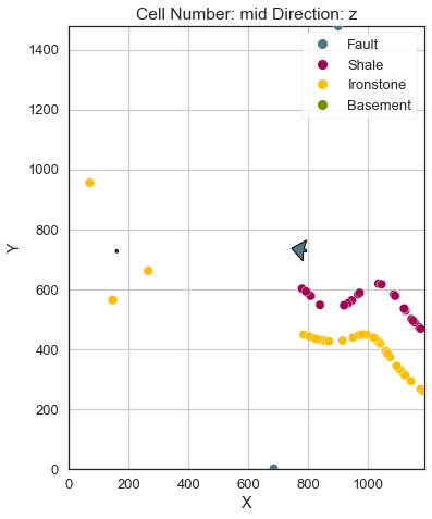
Interface Points of stratigraphic boundaries#

The interface points for this three point example will be digitized as points with the respective height value as given by the borehole information and the respective formation.

[10]:

import matplotlib.pyplot as plt
import matplotlib.image as mpimg
img = mpimg.imread('../images/interfaces_example15.png')
plt.figure(figsize=(10, 10))
imgplot = plt.imshow(img)
plt.axis('off')
plt.tight_layout()

../../_images/getting_started_example_example15_21_0.png

[11]:

interfaces = gpd.read_file(file_path + 'interfaces15.shp')
interfaces.head()

[11]:

	id	formation	Z	geometry
0	None	Shale	190	POINT (69.806 954.941)
1	None	Ironstone	170	POINT (69.806 954.941)
2	None	Ironstone	190	POINT (145.769 562.774)
3	None	Ironstone	185	POINT (264.746 660.701)
4	None	Shale	210	POINT (146.226 563.346)

Extracting Z coordinate from Digital Elevation Model#

[12]:

interfaces_coords = gg.vector.extract_xyz(gdf=interfaces, dem=None)
interfaces_coords

[12]:

	formation	Z	geometry	X	Y
0	Shale	190.00	POINT (69.806 954.941)	69.81	954.94
1	Ironstone	170.00	POINT (69.806 954.941)	69.81	954.94
2	Ironstone	190.00	POINT (145.769 562.774)	145.77	562.77
3	Ironstone	185.00	POINT (264.746 660.701)	264.75	660.70
4	Shale	210.00	POINT (146.226 563.346)	146.23	563.35
5	Shale	205.00	POINT (264.746 660.701)	264.75	660.70

[13]:

fault = gpd.read_file(file_path + 'fault15.shp')
fault = gg.vector.extract_xyz(gdf=fault, dem=topo_raster)
fault

[13]:

	formation	geometry	X	Y	Z
0	Fault	POINT (683.911 0.608)	683.91	0.61	178.76
1	Fault	POINT (899.671 1477.524)	899.67	1477.52	254.62

[14]:

import pandas as pd

interfaces_coords = pd.concat([interfaces_coords, fault]).reset_index()
interfaces_coords

[14]:

	index	formation	Z	geometry	X	Y
0	0	Shale	190.00	POINT (69.806 954.941)	69.81	954.94
1	1	Ironstone	170.00	POINT (69.806 954.941)	69.81	954.94
2	2	Ironstone	190.00	POINT (145.769 562.774)	145.77	562.77
3	3	Ironstone	185.00	POINT (264.746 660.701)	264.75	660.70
4	4	Shale	210.00	POINT (146.226 563.346)	146.23	563.35
5	5	Shale	205.00	POINT (264.746 660.701)	264.75	660.70
6	0	Fault	178.76	POINT (683.911 0.608)	683.91	0.61
7	1	Fault	254.62	POINT (899.671 1477.524)	899.67	1477.52

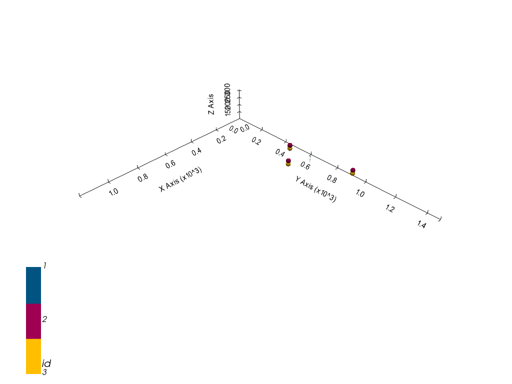
Plotting the Interface Points#

[15]:

fig, ax = plt.subplots(1, figsize=(10, 10))

interfaces.plot(ax=ax, column='formation', legend=True, aspect='equal')
interfaces_coords.plot(ax=ax, column='formation', legend=True, aspect='equal')
plt.grid()
ax.set_xlabel('X [m]')
ax.set_ylabel('Y [m]')
ax.set_xlim(0, 1187)
ax.set_ylim(0, 1479)

[15]:

(0.0, 1479.0)

../../_images/getting_started_example_example15_28_1.png

Orientations from Strike Lines#

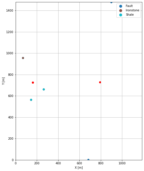
For this three point example, an orientation is calculated using gg.vector.calculate_orientation_for_three_point_problem().

[16]:

import matplotlib.pyplot as plt
import matplotlib.image as mpimg
img = mpimg.imread('../images/orientations_example15.png')
plt.figure(figsize=(10, 10))
imgplot = plt.imshow(img)
plt.axis('off')
plt.tight_layout()

../../_images/getting_started_example_example15_30_0.png

[17]:

orientations1 = gpd.read_file(file_path + 'interfaces15.shp')
orientations1 = orientations1[orientations1['formation']=='Ironstone']
orientations1

[17]:

	id	formation	Z	geometry
1	None	Ironstone	170	POINT (69.806 954.941)
2	None	Ironstone	190	POINT (145.769 562.774)
3	None	Ironstone	185	POINT (264.746 660.701)

[18]:

orientations1 = gg.vector.calculate_orientation_for_three_point_problem(gdf=orientations1)
orientations1

[18]:

	Z	formation	azimuth	dip	polarity	X	Y	geometry
0	181.67	Ironstone	-179.95	177.08	1	160.11	726.14	POINT (160.107 726.139)

Changing the Data Type of Fields#

[19]:

orientations1['Z'] = orientations1['Z'].astype(float)
orientations1['azimuth'] = orientations1['azimuth'].astype(float)
orientations1['dip'] = orientations1['dip'].astype(float)
orientations1['dip'] = 180 - orientations1['dip']
orientations1['azimuth'] = 180 - orientations1['azimuth']
orientations1['polarity'] = orientations1['polarity'].astype(float)
orientations1['X'] = orientations1['X'].astype(float)
orientations1['Y'] = orientations1['Y'].astype(float)
orientations1.info()

<class 'geopandas.geodataframe.GeoDataFrame'>
RangeIndex: 1 entries, 0 to 0
Data columns (total 8 columns):
 #   Column     Non-Null Count  Dtype
---  ------     --------------  -----
 0   Z          1 non-null      float64
 1   formation  1 non-null      object
 2   azimuth    1 non-null      float64
 3   dip        1 non-null      float64
 4   polarity   1 non-null      float64
 5   X          1 non-null      float64
 6   Y          1 non-null      float64
 7   geometry   1 non-null      geometry
dtypes: float64(6), geometry(1), object(1)
memory usage: 192.0+ bytes

[20]:

orientations2 = gpd.read_file(file_path + 'interfaces15.shp')
orientations2 = orientations2[orientations2['formation']=='Shale']
orientations2

[20]:

	id	formation	Z	geometry
0	None	Shale	190	POINT (69.806 954.941)
4	None	Shale	210	POINT (146.226 563.346)
5	None	Shale	205	POINT (264.746 660.701)

[21]:

orientations2 = gg.vector.calculate_orientation_for_three_point_problem(gdf=orientations2)
orientations2

[21]:

	Z	formation	azimuth	dip	polarity	X	Y	geometry
0	201.67	Shale	-179.77	177.07	1	160.26	726.33	POINT (160.259 726.329)

Changing the Data Type of Fields#

[22]:

orientations2['Z'] = orientations2['Z'].astype(float)
orientations2['azimuth'] = orientations2['azimuth'].astype(float)
orientations2['dip'] = orientations2['dip'].astype(float)
orientations2['dip'] = 180 - orientations2['dip']
orientations2['azimuth'] = 180 - orientations2['azimuth']
orientations2['polarity'] = orientations2['polarity'].astype(float)
orientations2['X'] = orientations2['X'].astype(float)
orientations2['Y'] = orientations2['Y'].astype(float)
orientations2.info()

<class 'geopandas.geodataframe.GeoDataFrame'>
RangeIndex: 1 entries, 0 to 0
Data columns (total 8 columns):
 #   Column     Non-Null Count  Dtype
---  ------     --------------  -----
 0   Z          1 non-null      float64
 1   formation  1 non-null      object
 2   azimuth    1 non-null      float64
 3   dip        1 non-null      float64
 4   polarity   1 non-null      float64
 5   X          1 non-null      float64
 6   Y          1 non-null      float64
 7   geometry   1 non-null      geometry
dtypes: float64(6), geometry(1), object(1)
memory usage: 192.0+ bytes

[23]:

orientations_fault = gpd.read_file(file_path + 'orientations15_fault.shp')
orientations_fault = gg.vector.extract_xyz(gdf=orientations_fault, dem=topo_raster)
orientations_fault

[23]:

	formation	dip	azimuth	polarity	geometry	X	Y	Z
0	Fault	90.00	280.00	1.00	POINT (792.591 727.511)	792.59	727.51	215.87

Merging Orientations#

[24]:

orientations = pd.concat([orientations1, orientations2, orientations_fault]).reset_index()
orientations

[24]:

	Z	formation	azimuth	dip	polarity	X	Y	geometry
0	181.67	Ironstone	359.95	2.92	1.00	160.11	726.14	POINT (160.107 726.139)
1	201.67	Shale	359.77	2.93	1.00	160.26	726.33	POINT (160.259 726.329)
2	215.87	Fault	280.00	90.00	1.00	792.59	727.51	POINT (792.591 727.511)

Plotting the Orientations#

[25]:

fig, ax = plt.subplots(1, figsize=(10,10))

interfaces.plot(ax=ax, column='formation', legend=True, aspect='equal')
interfaces_coords.plot(ax=ax, column='formation', legend=True, aspect='equal')
orientations.plot(ax=ax, color='red', aspect='equal')
plt.grid()
plt.xlim(0,1187)
plt.ylim(0,1479)
plt.xlabel('X [m]')
plt.ylabel('Y [m]')

[25]:

Text(179.77829589465532, 0.5, 'Y [m]')

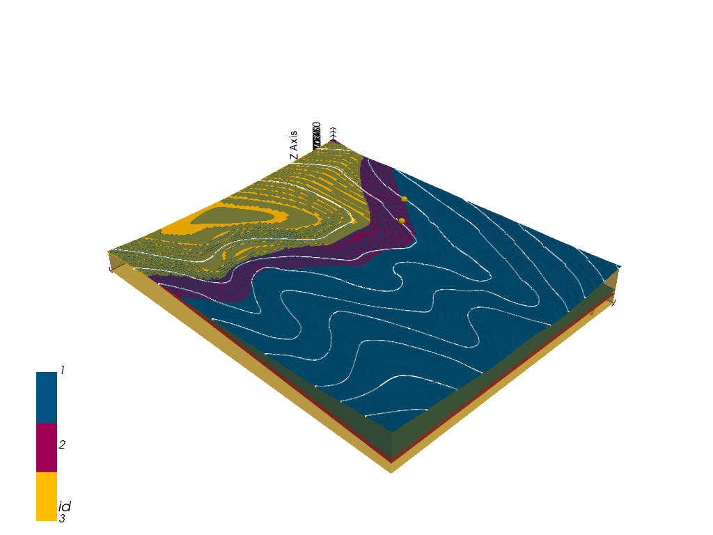
../../_images/getting_started_example_example15_43_1.png

GemPy Model Construction (Part A)#

The structural geological model will be constructed using the GemPy package. The first model is calculated without the fault.

[26]:

import gempy as gp

WARNING (theano.configdefaults): g++ not available, if using conda: `conda install m2w64-toolchain`
WARNING (theano.configdefaults): g++ not detected ! Theano will be unable to execute optimized C-implementations (for both CPU and GPU) and will default to Python implementations. Performance will be severely degraded. To remove this warning, set Theano flags cxx to an empty string.
WARNING (theano.tensor.blas): Using NumPy C-API based implementation for BLAS functions.

Creating New Model#

[27]:

geo_model = gp.create_model('Model15a')
geo_model

[27]:

Model15a  2022-04-05 11:07

Initiate Data#

The fault interfaces and orientations will be removed from the first model to model the layers also beyond the fault. As the information is provided that the fault has an offset of 20 m, the layers will be exported, the boundaries will be digitized and the elevation will be reduced by 20 m.

[28]:

interfaces_coords_new=interfaces_coords[interfaces_coords['formation'] != 'Fault']
interfaces_coords_new

[28]:

	index	formation	Z	geometry	X	Y
0	0	Shale	190.00	POINT (69.806 954.941)	69.81	954.94
1	1	Ironstone	170.00	POINT (69.806 954.941)	69.81	954.94
2	2	Ironstone	190.00	POINT (145.769 562.774)	145.77	562.77
3	3	Ironstone	185.00	POINT (264.746 660.701)	264.75	660.70
4	4	Shale	210.00	POINT (146.226 563.346)	146.23	563.35
5	5	Shale	205.00	POINT (264.746 660.701)	264.75	660.70

[29]:

orientations_new=orientations[orientations['formation'] != 'Fault']
orientations_new

[29]:

	index	Z	formation	azimuth	dip	polarity	X	Y	geometry
0	0	181.67	Ironstone	359.95	2.92	1.00	160.11	726.14	POINT (160.107 726.139)
1	0	201.67	Shale	359.77	2.93	1.00	160.26	726.33	POINT (160.259 726.329)

[30]:

gp.init_data(geo_model, [0, 1187, 0, 1479, 100, 300], [100, 100, 100],
             surface_points_df=interfaces_coords_new[interfaces_coords_new['Z'] != 0],
             orientations_df=orientations_new,
             default_values=True)

Active grids: ['regular']

[30]:

Model15a  2022-04-05 11:07

Model Surfaces#

[31]:

geo_model.surfaces

[31]:

	surface	series	order_surfaces	color	id
0	Shale	Default series	1	#015482	1
1	Ironstone	Default series	2	#9f0052	2

Mapping the Stack to Surfaces#

[32]:

gp.map_stack_to_surfaces(geo_model,
                         {
                          'Strata1': ('Shale', 'Ironstone'),
                         },
                         remove_unused_series=True)
geo_model.add_surfaces('Basement')

[32]:

	surface	series	order_surfaces	color	id
0	Shale	Strata1	1	#015482	1
1	Ironstone	Strata1	2	#9f0052	2
2	Basement	Strata1	3	#ffbe00	3

Showing the Number of Data Points#

[33]:

gg.utils.show_number_of_data_points(geo_model=geo_model)

[33]:

	surface	series	order_surfaces	color	id	No. of Interfaces	No. of Orientations
0	Shale	Strata1	1	#015482	1	3	1
1	Ironstone	Strata1	2	#9f0052	2	3	1
2	Basement	Strata1	3	#ffbe00	3	0	0

Loading Digital Elevation Model#

[34]:

geo_model.set_topography(
    source='gdal', filepath=file_path + 'raster15.tif')

Cropped raster to geo_model.grid.extent.
depending on the size of the raster, this can take a while...
storing converted file...
Active grids: ['regular' 'topography']

[34]:

Grid Object. Values:
array([[   5.935     ,    7.395     ,  101.        ],
       [   5.935     ,    7.395     ,  103.        ],
       [   5.935     ,    7.395     ,  105.        ],
       ...,
       [1184.49578059, 1466.50844595,  275.3008728 ],
       [1184.49578059, 1471.50506757,  275.80532837],
       [1184.49578059, 1476.50168919,  276.31124878]])

Plotting Input Data#

[35]:

gp.plot_2d(geo_model, direction='z', show_lith=False, show_boundaries=False)
plt.grid()

../../_images/getting_started_example_example15_61_0.png

[36]:

gp.plot_3d(geo_model, image=False, plotter_type='basic', notebook=True)

../../_images/getting_started_example_example15_62_0.png

[36]:

<gempy.plot.vista.GemPyToVista at 0x1e68be5d250>

Setting the Interpolator#

[37]:

gp.set_interpolator(geo_model,
                    compile_theano=True,
                    theano_optimizer='fast_compile',
                    verbose=[],
                    update_kriging=False
                    )

Compiling theano function...
Level of Optimization:  fast_compile
Device:  cpu
Precision:  float64
Number of faults:  0
Compilation Done!
Kriging values:
                   values
range            1906.94
$C_o$           86581.19
drift equations      [3]

[37]:

<gempy.core.interpolator.InterpolatorModel at 0x1e685ddafd0>

Computing Model#

[38]:

sol = gp.compute_model(geo_model, compute_mesh=True)

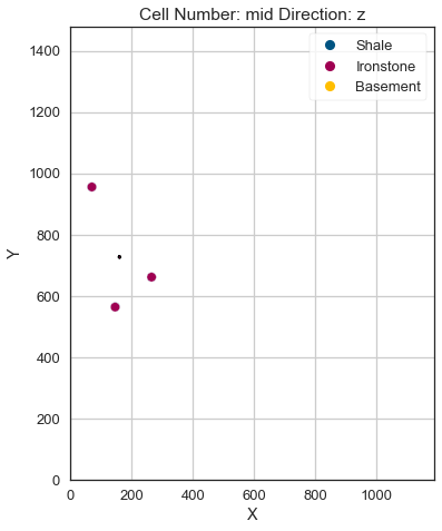
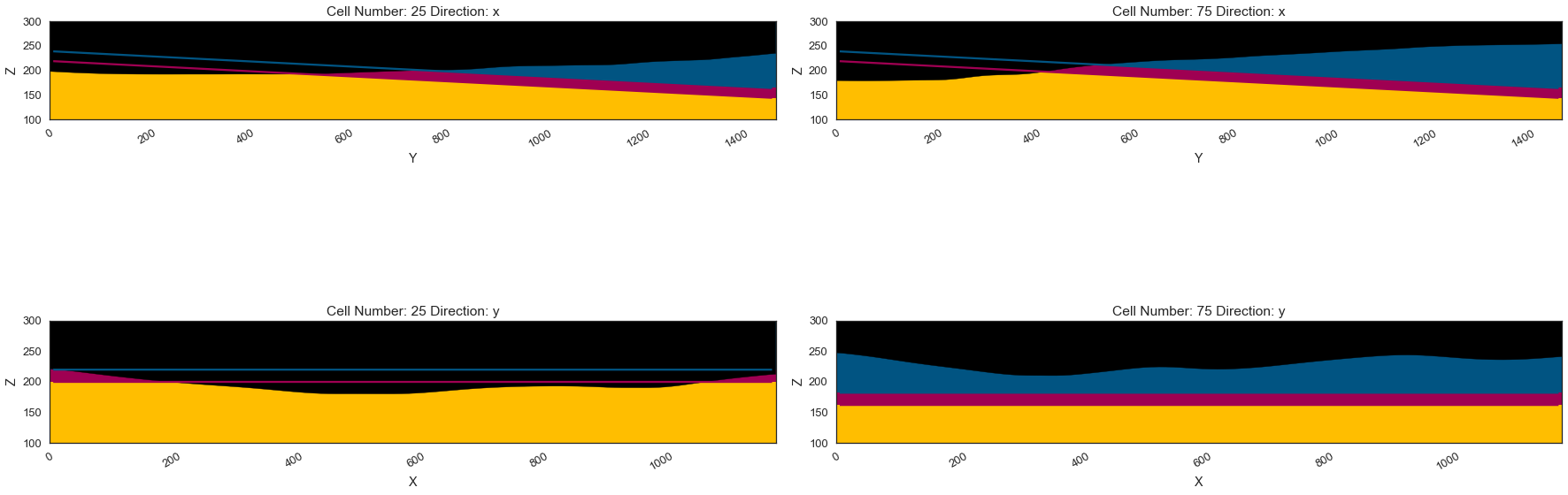
Plotting Cross Sections#

[39]:

gp.plot_2d(geo_model, direction=['x', 'x', 'y', 'y'], cell_number=[25, 75, 25, 75], show_topography=True, show_data=False)

[39]:

<gempy.plot.visualization_2d.Plot2D at 0x1e68a3e4a90>

../../_images/getting_started_example_example15_68_1.png

Plotting 3D Model#

[40]:

gpv = gp.plot_3d(geo_model, image=False, show_topography=True,
                 plotter_type='basic', notebook=True, show_lith=True)

../../_images/getting_started_example_example15_70_0.png

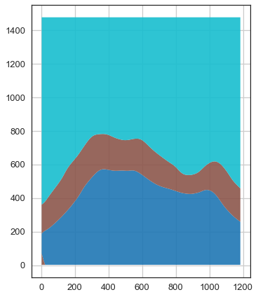
Creating Polygons from GemPy Model#

A GeoDataFrame containing polygons representing the geological map can be created using gg.post.extract_lithologies(). This data is now being saved and the constructed layer boundaries beyond the fault in the east are being digitized. Their elevation values will be reduced by 20 m to simulate the offset of the fault. The model will then be recalculated again.

[41]:

gdf = gg.post.extract_lithologies(geo_model, [0, 1187, 0, 1479], 'EPSG:4326')
gdf

[41]:

	formation	geometry
0	Basement	POLYGON ((22.538 3.254, 22.804 2.498, 27.546 2...
1	Ironstone	POLYGON ((7.513 2.498, 12.521 2.498, 17.530 2....
2	Ironstone	POLYGON ((5.851 192.370, 7.513 194.147, 10.887...
3	Shale	POLYGON ((4.134 362.255, 7.513 365.081, 10.021...

[42]:

gdf = gpd.read_file(file_path + 'geolmap.shp')
gdf

[42]:

	formation	geometry
0	Conglomerate	POLYGON ((22.538 3.254, 21.064 7.495, 19.356 1...
1	Ironstone	POLYGON ((7.513 2.498, 2.504 2.498, 2.504 7.49...
2	Ironstone	POLYGON ((5.851 192.370, 2.504 188.069, 2.504 ...
3	Shale	POLYGON ((4.134 362.255, 2.504 360.939, 2.504 ...

[43]:

gdf.plot(column='formation',  alpha=0.9, aspect='equal')
plt.grid()

../../_images/getting_started_example_example15_74_0.png

Preparing Interfaces beyond the fault#

[44]:

interfaces_beyond_fault =  gpd.read_file(file_path + 'interfaces15_beyond_fault.shp')
interfaces_beyond_fault = gg.vector.extract_xyz(gdf=interfaces_beyond_fault, dem=topo_raster)
interfaces_beyond_fault

[44]:

	formation	geometry	X	Y	Z
0	Shale	POINT (778.812 601.522)	778.81	601.52	208.06
1	Shale	POINT (783.821 597.991)	783.82	597.99	208.15
2	Shale	POINT (788.829 594.245)	788.83	594.25	208.26
3	Shale	POINT (791.557 592.100)	791.56	592.10	208.71
4	Shale	POINT (797.430 587.103)	797.43	587.10	208.89
...	...	...	...	...	...
250	Ironstone	POINT (1169.470 270.001)	1169.47	270.00	205.13
251	Ironstone	POINT (1172.985 267.319)	1172.99	267.32	205.24
252	Ironstone	POINT (1174.479 266.187)	1174.48	266.19	205.24
253	Ironstone	POINT (1179.487 262.439)	1179.49	262.44	205.33
254	Ironstone	POINT (1184.496 258.751)	1184.50	258.75	205.42

255 rows × 5 columns

Substracting the fault offset#

[45]:

interfaces_beyond_fault['Z']=interfaces_beyond_fault['Z']-20
interfaces_beyond_fault

[45]:

	formation	geometry	X	Y	Z
0	Shale	POINT (778.812 601.522)	778.81	601.52	188.06
1	Shale	POINT (783.821 597.991)	783.82	597.99	188.15
2	Shale	POINT (788.829 594.245)	788.83	594.25	188.26
3	Shale	POINT (791.557 592.100)	791.56	592.10	188.71
4	Shale	POINT (797.430 587.103)	797.43	587.10	188.89
...	...	...	...	...	...
250	Ironstone	POINT (1169.470 270.001)	1169.47	270.00	185.13
251	Ironstone	POINT (1172.985 267.319)	1172.99	267.32	185.24
252	Ironstone	POINT (1174.479 266.187)	1174.48	266.19	185.24
253	Ironstone	POINT (1179.487 262.439)	1179.49	262.44	185.33
254	Ironstone	POINT (1184.496 258.751)	1184.50	258.75	185.42

255 rows × 5 columns

Mergin old and new interfaces#

[46]:

interfaces_coords = pd.concat([interfaces_coords, interfaces_beyond_fault.sample(n=50)]).reset_index()
interfaces_coords

[46]:

	level_0	index	formation	Z	geometry	X	Y
0	0	0.00	Shale	190.00	POINT (69.806 954.941)	69.81	954.94
1	1	1.00	Ironstone	170.00	POINT (69.806 954.941)	69.81	954.94
2	2	2.00	Ironstone	190.00	POINT (145.769 562.774)	145.77	562.77
3	3	3.00	Ironstone	185.00	POINT (264.746 660.701)	264.75	660.70
4	4	4.00	Shale	210.00	POINT (146.226 563.346)	146.23	563.35
5	5	5.00	Shale	205.00	POINT (264.746 660.701)	264.75	660.70
6	6	0.00	Fault	178.76	POINT (683.911 0.608)	683.91	0.61
7	7	1.00	Fault	254.62	POINT (899.671 1477.524)	899.67	1477.52
8	177	NaN	Ironstone	176.27	POINT (949.099 437.906)	949.10	437.91
9	199	NaN	Ironstone	177.36	POINT (1039.795 417.218)	1039.79	417.22
10	156	NaN	Ironstone	176.90	POINT (853.939 427.352)	853.94	427.35
11	127	NaN	Shale	194.60	POINT (1169.470 472.641)	1169.47	472.64
12	4	NaN	Shale	188.89	POINT (797.430 587.103)	797.43	587.10
13	230	NaN	Ironstone	182.46	POINT (1114.378 320.613)	1114.38	320.61
14	155	NaN	Ironstone	176.77	POINT (848.930 428.164)	848.93	428.16
15	196	NaN	Ironstone	177.05	POINT (1034.243 423.251)	1034.24	423.25
16	110	NaN	Shale	191.82	POINT (1124.395 527.284)	1124.39	527.28
17	0	NaN	Shale	188.06	POINT (778.812 601.522)	778.81	601.52
18	20	NaN	Shale	190.81	POINT (838.823 547.130)	838.82	547.13
19	74	NaN	Shale	187.12	POINT (1034.243 618.288)	1034.24	618.29
20	92	NaN	Shale	188.89	POINT (1085.673 582.106)	1085.67	582.11
21	138	NaN	Ironstone	175.84	POINT (783.821 447.680)	783.82	447.68
22	119	NaN	Shale	193.19	POINT (1144.428 499.461)	1144.43	499.46
23	94	NaN	Shale	189.24	POINT (1089.653 577.110)	1089.65	577.11
24	77	NaN	Shale	187.33	POINT (1044.259 616.032)	1044.26	616.03
25	123	NaN	Shale	193.80	POINT (1154.445 488.152)	1154.45	488.15
26	53	NaN	Shale	189.23	POINT (965.782 582.106)	965.78	582.11
27	8	NaN	Shale	189.40	POINT (807.567 577.110)	807.57	577.11
28	194	NaN	Ironstone	176.60	POINT (1024.226 432.683)	1024.23	432.68
29	160	NaN	Ironstone	177.25	POINT (868.964 425.396)	868.96	425.40
30	181	NaN	Ironstone	176.12	POINT (969.133 446.025)	969.13	446.03
31	55	NaN	Shale	189.01	POINT (971.197 587.103)	971.20	587.10
32	233	NaN	Ironstone	183.05	POINT (1122.155 312.289)	1122.16	312.29
33	241	NaN	Ironstone	184.02	POINT (1142.482 292.302)	1142.48	292.30
34	144	NaN	Ironstone	176.33	POINT (803.854 440.894)	803.85	440.89
35	252	NaN	Ironstone	185.24	POINT (1174.479 266.187)	1174.48	266.19
36	152	NaN	Ironstone	176.80	POINT (833.905 431.359)	833.91	431.36
37	3	NaN	Shale	188.71	POINT (791.557 592.100)	791.56	592.10
38	129	NaN	Shale	194.85	POINT (1174.933 467.184)	1174.93	467.18
39	46	NaN	Shale	190.13	POINT (944.754 562.120)	944.75	562.12
40	169	NaN	Ironstone	176.79	POINT (914.040 427.799)	914.04	427.80
41	211	NaN	Ironstone	179.46	POINT (1069.302 377.432)	1069.30	377.43
42	186	NaN	Ironstone	175.71	POINT (989.167 448.328)	989.17	448.33
43	206	NaN	Ironstone	178.75	POINT (1059.017 392.235)	1059.02	392.23
44	149	NaN	Ironstone	176.38	POINT (823.888 434.155)	823.89	434.15
45	212	NaN	Ironstone	179.93	POINT (1072.891 372.248)	1072.89	372.25
46	225	NaN	Ironstone	181.85	POINT (1103.757 332.275)	1103.76	332.28
47	187	NaN	Ironstone	175.83	POINT (994.175 447.621)	994.18	447.62
48	42	NaN	Shale	190.77	POINT (931.344 552.127)	931.34	552.13
49	109	NaN	Shale	191.38	POINT (1121.307 532.140)	1121.31	532.14
50	108	NaN	Shale	191.45	POINT (1119.386 535.097)	1119.39	535.10
51	38	NaN	Shale	191.03	POINT (919.049 545.720)	919.05	545.72
52	192	NaN	Ironstone	176.51	POINT (1018.269 437.204)	1018.27	437.20
53	121	NaN	Shale	193.50	POINT (1149.437 493.655)	1149.44	493.66
54	254	NaN	Ironstone	185.42	POINT (1184.496 258.751)	1184.50	258.75
55	222	NaN	Ironstone	181.17	POINT (1094.344 343.135)	1094.34	343.14
56	184	NaN	Ironstone	175.73	POINT (979.150 448.200)	979.15	448.20
57	209	NaN	Ironstone	178.98	POINT (1064.293 384.655)	1064.29	384.65

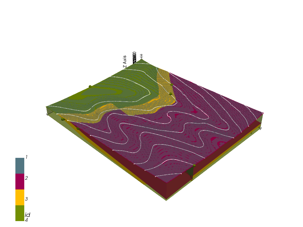
GemPy Model Construction (Part B)#

The structural geological model will be constructed using the GemPy package.

[47]:

import gempy as gp

Creating new Model#

[48]:

geo_model = gp.create_model('Model15b')
geo_model

[48]:

Model15b  2022-04-05 11:08

Initiate Data#

[49]:

gp.init_data(geo_model, [0, 1187, 0, 1479, 100, 300], [100, 100, 100],
             surface_points_df=interfaces_coords[interfaces_coords['Z'] != 0],
             orientations_df=orientations,
             default_values=True)

Active grids: ['regular']

[49]:

Model15b  2022-04-05 11:08

Model Surfaces#

[50]:

geo_model.surfaces

[50]:

	surface	series	order_surfaces	color	id
0	Shale	Default series	1	#015482	1
1	Ironstone	Default series	2	#9f0052	2
2	Fault	Default series	3	#ffbe00	3

Mapping the Stack to Surfaces#

[51]:

gp.map_stack_to_surfaces(geo_model,
                         {
                          'Fault1' : ('Fault'),
                          'Strata1': ('Shale', 'Ironstone'),
                         },
                         remove_unused_series=True)
geo_model.add_surfaces('Basement')
geo_model.set_is_fault(['Fault1'])

Fault colors changed. If you do not like this behavior, set change_color to False.

[51]:

	order_series	BottomRelation	isActive	isFault	isFinite
Fault1	1	Fault	True	True	False
Strata1	2	Erosion	True	False	False

Showing the Number of Data Points#

[52]:

gg.utils.show_number_of_data_points(geo_model=geo_model)

[52]:

	surface	series	order_surfaces	color	id	No. of Interfaces	No. of Orientations
2	Fault	Fault1	1	#527682	1	2	1
0	Shale	Strata1	1	#9f0052	2	25	1
1	Ironstone	Strata1	2	#ffbe00	3	31	1
3	Basement	Strata1	3	#728f02	4	0	0

Loading Digital Elevation Model#

[53]:

geo_model.set_topography(
    source='gdal', filepath=file_path + 'raster15.tif')

Cropped raster to geo_model.grid.extent.
depending on the size of the raster, this can take a while...
storing converted file...
Active grids: ['regular' 'topography']

[53]:

Grid Object. Values:
array([[   5.935     ,    7.395     ,  101.        ],
       [   5.935     ,    7.395     ,  103.        ],
       [   5.935     ,    7.395     ,  105.        ],
       ...,
       [1184.49578059, 1466.50844595,  275.3008728 ],
       [1184.49578059, 1471.50506757,  275.80532837],
       [1184.49578059, 1476.50168919,  276.31124878]])

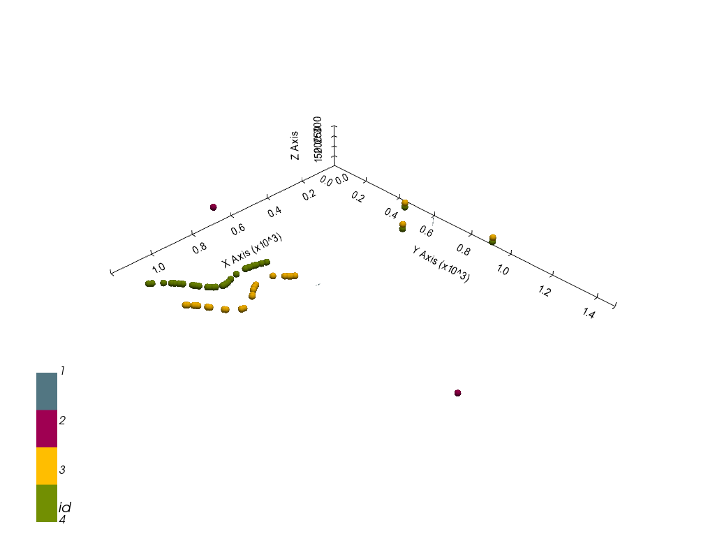
Plotting Input Data#

[54]:

gp.plot_2d(geo_model, direction='z', show_lith=False, show_boundaries=False)
plt.grid()

../../_images/getting_started_example_example15_96_0.png

[55]:

gp.plot_3d(geo_model, image=False, plotter_type='basic', notebook=True)

../../_images/getting_started_example_example15_97_0.png

[55]:

<gempy.plot.vista.GemPyToVista at 0x1e6886403d0>

Setting the Interpolator#

[56]:

gp.set_interpolator(geo_model,
                    compile_theano=True,
                    theano_optimizer='fast_compile',
                    verbose=[],
                    update_kriging = False
                    )

Compiling theano function...
Level of Optimization:  fast_compile
Device:  cpu
Precision:  float64
Number of faults:  1
Compilation Done!
Kriging values:
                   values
range            1906.94
$C_o$           86581.19
drift equations   [3, 3]

[56]:

<gempy.core.interpolator.InterpolatorModel at 0x1e687f7d370>

Computing Model#

[57]:

sol = gp.compute_model(geo_model, compute_mesh=True)

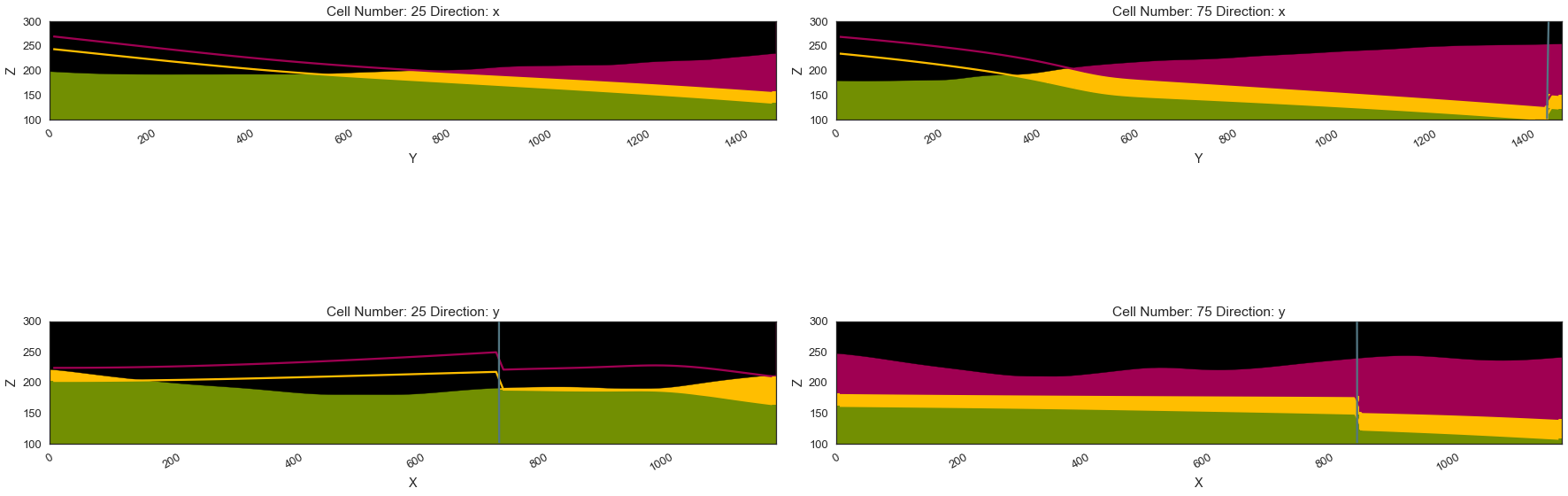
Plotting Cross Sections#

[58]:

gp.plot_2d(geo_model, direction=['x', 'x', 'y', 'y'], cell_number=[25, 75, 25, 75], show_topography=True, show_data=False)

[58]:

<gempy.plot.visualization_2d.Plot2D at 0x1e6b7bacbb0>

../../_images/getting_started_example_example15_103_1.png

Plotting 3D Model#

[59]:

gpv = gp.plot_3d(geo_model, image=False, show_topography=True,
                 plotter_type='basic', notebook=True, show_lith=True)

../../_images/getting_started_example_example15_105_0.png

[ ]:

GemGIS - Spatial data processing for geomodeling

Example 15 - Three Point Problem

Contents

Example 15 - Three Point Problem#

Licensing#

Import GemGIS#

Importing Libraries and loading Data#

Creating Digital Elevation Model from Contour Lines#

Interpolating the contour lines#

Plotting the raster#

Saving the raster to disc#

Opening Raster#

Interface Points of stratigraphic boundaries#

Extracting Z coordinate from Digital Elevation Model#

Plotting the Interface Points#

Orientations from Strike Lines#

Changing the Data Type of Fields#

Changing the Data Type of Fields#

Merging Orientations#

Plotting the Orientations#

GemPy Model Construction (Part A)#

Creating New Model#

Initiate Data#

Model Surfaces#

Mapping the Stack to Surfaces#

Showing the Number of Data Points#

Loading Digital Elevation Model#

Plotting Input Data#

Setting the Interpolator#

Computing Model#

Plotting Cross Sections#

Plotting 3D Model#

Creating Polygons from GemPy Model#

Preparing Interfaces beyond the fault#

Substracting the fault offset#

Mergin old and new interfaces#

GemPy Model Construction (Part B)#

Creating new Model#

Initiate Data#

Model Surfaces#

Mapping the Stack to Surfaces#

Showing the Number of Data Points#

Loading Digital Elevation Model#

Plotting Input Data#

Setting the Interpolator#

Computing Model#

Plotting Cross Sections#

Plotting 3D Model#