
Example 26 - Unconformable Folded Layers
Contents
Example 26 - Unconformable Folded Layers#
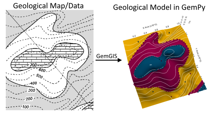
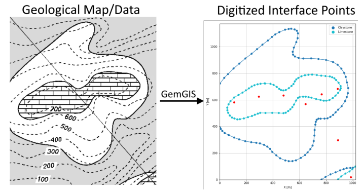
This example will show how to convert the geological map below using GemGIS to a GemPy model. This example is based on digitized data. The area is 1022 m wide (W-E extent) and 1172 m high (N-S extent). The model represents unconformable folded layers.
The map has been georeferenced with QGIS. The stratigraphic boundaries were digitized in QGIS. Strikes lines were digitized in QGIS as well and will be used to calculate orientations for the GemPy model. The contour lines were also digitized and will be interpolated with GemGIS to create a topography for the model.
Map Source: Unknown
[1]:
import matplotlib.pyplot as plt
import matplotlib.image as mpimg
img = mpimg.imread('../images/cover_example26.png')
plt.figure(figsize=(10, 10))
imgplot = plt.imshow(img)
plt.axis('off')
plt.tight_layout()
Licensing#
Computational Geosciences and Reservoir Engineering, RWTH Aachen University, Authors: Alexander Juestel. For more information contact: alexander.juestel(at)rwth-aachen.de
This work is licensed under a Creative Commons Attribution 4.0 International License (http://creativecommons.org/licenses/by/4.0/)
Import GemGIS#
If you have installed GemGIS via pip, you can import GemGIS like any other package. If you have downloaded the repository, append the path to the directory where the GemGIS repository is stored and then import GemGIS.
[2]:
import warnings
warnings.filterwarnings("ignore")
import gemgis as gg
Importing Libraries and loading Data#
All remaining packages can be loaded in order to prepare the data and to construct the model. The example data is downloaded form an external server using pooch. It will be stored in a data folder in the same directory where this notebook is stored.
[3]:
import geopandas as gpd
import rasterio
[4]:
file_path = 'data/example26/'
gg.download_gemgis_data.download_tutorial_data(filename="example26_unconformable_folded_layers.zip", dirpath=file_path)
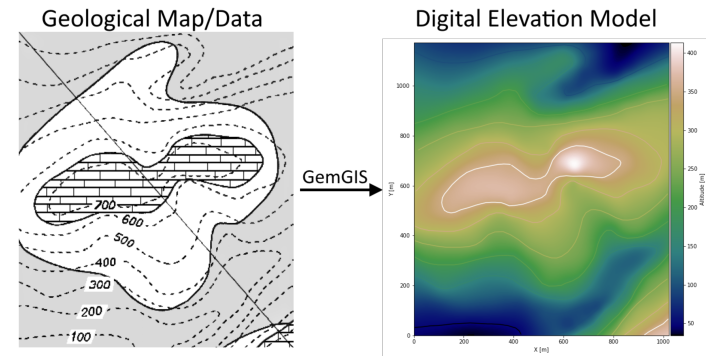
Creating Digital Elevation Model from Contour Lines#
The digital elevation model (DEM) will be created by interpolating contour lines digitized from the georeferenced map using the SciPy Radial Basis Function interpolation wrapped in GemGIS. The respective function used for that is gg.vector.interpolate_raster().
[5]:
import matplotlib.pyplot as plt
import matplotlib.image as mpimg
img = mpimg.imread('../images/dem_example26.png')
plt.figure(figsize=(10, 10))
imgplot = plt.imshow(img)
plt.axis('off')
plt.tight_layout()
[6]:
topo = gpd.read_file(file_path + 'topo26.shp')
topo['Z'] = topo['Z']*0.5
topo.head()
[6]:
| id | Z | geometry | |
|---|---|---|---|
| 0 | None | 50.00 | LINESTRING (1.874 31.940, 31.950 34.114, 67.10... |
| 1 | None | 100.00 | LINESTRING (2.961 153.696, 32.675 153.696, 65.... |
| 2 | None | 350.00 | LINESTRING (924.099 1.864, 942.217 14.546, 974... |
| 3 | None | 300.00 | LINESTRING (844.378 1.139, 873.367 23.606, 899... |
| 4 | None | 250.00 | LINESTRING (793.284 1.864, 816.113 29.766, 834... |
Interpolating the contour lines#
[7]:
topo_raster = gg.vector.interpolate_raster(gdf=topo, value='Z', method='rbf', res=5)
Plotting the raster#
[8]:
import matplotlib.pyplot as plt

from mpl_toolkits.axes_grid1 import make_axes_locatable

fix, ax = plt.subplots(1, figsize=(10,10))
topo.plot(ax=ax, aspect='equal', column='Z', cmap='gist_earth')
im = ax.imshow(topo_raster, origin='lower', extent=[0,1022,0,1172], cmap='gist_earth')
divider = make_axes_locatable(ax)
cax = divider.append_axes("right", size="5%", pad=0.05)
cbar = plt.colorbar(im, cax=cax)
cbar.set_label('Altitude [m]')
ax.set_xlabel('X [m]')
ax.set_ylabel('Y [m]')
[8]:
Text(94.3788293897884, 0.5, 'Y [m]')
Saving the raster to disc#
After the interpolation of the contour lines, the raster is saved to disc using gg.raster.save_as_tiff(). The function will not be executed as as raster is already provided with the example data.
Opening Raster#
The previously computed and saved raster can now be opened using rasterio.
[9]:
topo_raster = rasterio.open(file_path + 'raster26.tif')
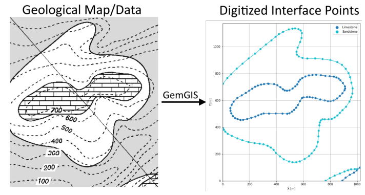
Interface Points of stratigraphic boundaries#
The interface points will be extracted from LineStrings digitized from the georeferenced map using QGIS. It is important to provide a formation name for each layer boundary. The vertical position of the interface point will be extracted from the digital elevation model using the GemGIS function gg.vector.extract_xyz(). The resulting GeoDataFrame now contains single points including the information about the respective formation.
[10]:
import matplotlib.pyplot as plt
import matplotlib.image as mpimg
img = mpimg.imread('../images/interfaces_example26.png')
plt.figure(figsize=(10, 10))
imgplot = plt.imshow(img)
plt.axis('off')
plt.tight_layout()
[11]:
interfaces = gpd.read_file(file_path + 'interfaces26.shp')
interfaces.head()
[11]:
| id | formation | geometry | |
|---|---|---|---|
| 0 | None | Limestone | LINESTRING (341.774 722.613, 381.997 720.438, ... |
| 1 | None | Limestone | LINESTRING (890.761 2.226, 914.315 24.330, 945... |
| 2 | None | Claystone | LINESTRING (765.744 0.777, 796.546 20.707, 833... |
| 3 | None | Claystone | LINESTRING (2.236 722.975, 34.487 765.010, 62.... |
Extracting XY coordinates from Digital Elevation Model#
[12]:
interfaces_coords = gg.vector.extract_xyz(gdf=interfaces, dem=topo_raster)
interfaces_coords = interfaces_coords.sort_values(by='formation', ascending=False)
interfaces_coords.head()
[12]:
| formation | geometry | X | Y | Z | |
|---|---|---|---|---|---|
| 0 | Limestone | POINT (341.774 722.613) | 341.77 | 722.61 | 338.52 |
| 54 | Limestone | POINT (287.057 496.133) | 287.06 | 496.13 | 312.83 |
| 62 | Limestone | POINT (92.828 466.781) | 92.83 | 466.78 | 329.27 |
| 61 | Limestone | POINT (110.946 459.896) | 110.95 | 459.90 | 328.27 |
| 60 | Limestone | POINT (132.688 453.011) | 132.69 | 453.01 | 325.96 |
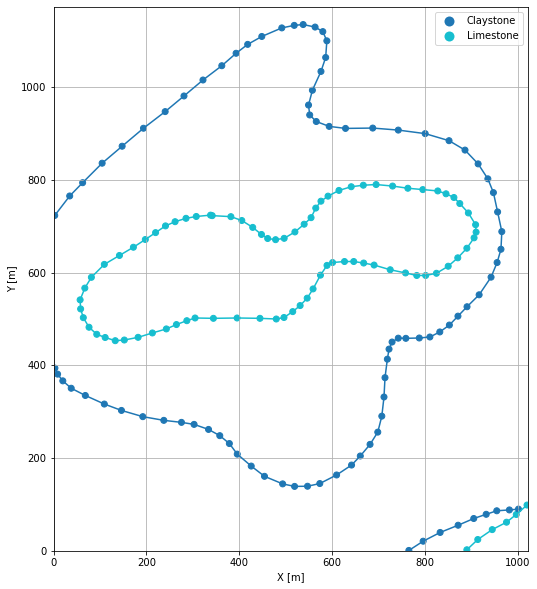
Plotting the Interface Points#
[13]:
fig, ax = plt.subplots(1, figsize=(10,10))

interfaces.plot(ax=ax, column='formation', legend=True, aspect='equal')
interfaces_coords.plot(ax=ax, column='formation', legend=True, aspect='equal')
plt.grid()
plt.xlabel('X [m]')
plt.ylabel('Y [m]')
plt.xlim(0,1022)
plt.ylim(0,1172)
[13]:
(0.0, 1172.0)
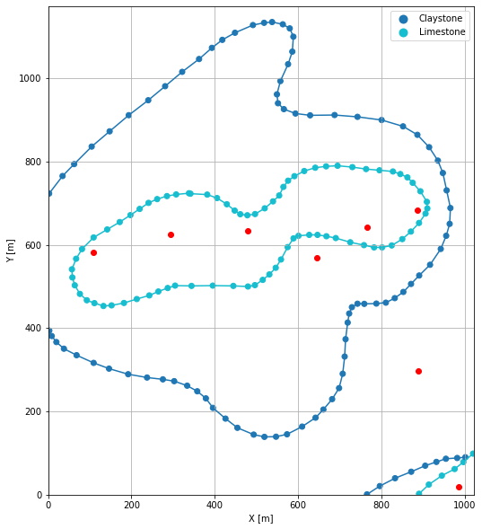
Orientations from Strike Lines#
Strike lines connect outcropping stratigraphic boundaries (interfaces) of the same altitude. In other words: the intersections between topographic contours and stratigraphic boundaries at the surface. The height difference and the horizontal difference between two digitized lines is used to calculate the dip and azimuth and hence an orientation that is necessary for GemPy. In order to calculate the orientations, each set of strikes lines/LineStrings for one formation must be given an id
number next to the altitude of the strike line. The id field is already predefined in QGIS. The strike line with the lowest altitude gets the id number 1, the strike line with the highest altitude the the number according to the number of digitized strike lines. It is currently recommended to use one set of strike lines for each structural element of one formation as illustrated.
[14]:
import matplotlib.pyplot as plt
import matplotlib.image as mpimg
img = mpimg.imread('../images/orientations_example26.png')
plt.figure(figsize=(10, 10))
imgplot = plt.imshow(img)
plt.axis('off')
plt.tight_layout()
[15]:
strikes = gpd.read_file(file_path + 'strikes26.shp')
strikes['Z'] = strikes['Z']*0.5
strikes
[15]:
| id | formation | Z | geometry | |
|---|---|---|---|---|
| 0 | 2 | Limestone2 | 350.00 | LINESTRING (208.061 655.212, 205.887 509.540) |
| 1 | 1 | Limestone2 | 350.00 | LINESTRING (750.887 734.208, 750.887 632.021) |
| 2 | 4 | Claystone1 | 300.00 | LINESTRING (953.088 757.400, 950.914 613.178) |
| 3 | 3 | Claystone1 | 250.00 | LINESTRING (823.361 895.099, 821.911 464.607) |
| 4 | 2 | Limestone1 | 350.00 | LINESTRING (962.510 24.693, 963.235 0.052) |
| 5 | 1 | Limestone1 | 350.00 | LINESTRING (1009.618 51.508, 1009.618 2.226) |
| 6 | 2 | Claystone1 | 200.00 | LINESTRING (712.476 909.594, 707.403 296.468) |
| 7 | 1 | Claystone1 | 150.00 | LINESTRING (587.097 917.566, 576.226 147.898) |
| 8 | 1 | Claystone2 | 150.00 | LINESTRING (387.070 1070.485, 385.621 221.096) |
| 9 | 2 | Claystone2 | 200.00 | LINESTRING (202.988 919.016, 199.364 287.047) |
| 10 | 3 | Claystone2 | 250.00 | LINESTRING (16.006 744.355, 12.382 374.740) |
| 11 | 1 | Claystone3 | 250.00 | LINESTRING (822.636 462.433, 821.187 34.114) |
| 12 | 2 | Claystone3 | 300.00 | LINESTRING (951.639 606.655, 955.987 85.570) |
Calculate Orientations for each formation#
[16]:
orientations_claystone1 = gg.vector.calculate_orientations_from_strike_lines(gdf=strikes[strikes['formation']=='Claystone1'].sort_values(by='Z', ascending=True).reset_index())
orientations_claystone1
[16]:
| dip | azimuth | Z | geometry | polarity | formation | X | Y | |
|---|---|---|---|---|---|---|---|---|
| 0 | 21.73 | 270.68 | 175.00 | POINT (645.801 567.882) | 1.00 | Claystone1 | 645.80 | 567.88 |
| 1 | 24.25 | 270.38 | 225.00 | POINT (766.288 641.442) | 1.00 | Claystone1 | 766.29 | 641.44 |
| 2 | 21.26 | 270.26 | 275.00 | POINT (887.319 682.571) | 1.00 | Claystone1 | 887.32 | 682.57 |
[17]:
orientations_claystone2 = gg.vector.calculate_orientations_from_strike_lines(gdf=strikes[strikes['formation']=='Claystone2'].sort_values(by='Z', ascending=True).reset_index())
orientations_claystone2
[17]:
| dip | azimuth | Z | geometry | polarity | formation | X | Y | |
|---|---|---|---|---|---|---|---|---|
| 0 | 15.22 | 90.18 | 175.00 | POINT (293.761 624.411) | 1.00 | Claystone2 | 293.76 | 624.41 |
| 1 | 15.05 | 90.39 | 225.00 | POINT (107.685 581.289) | 1.00 | Claystone2 | 107.68 | 581.29 |
[18]:
orientations_claystone3 = gg.vector.calculate_orientations_from_strike_lines(gdf=strikes[strikes['formation']=='Claystone3'].sort_values(by='Z', ascending=True).reset_index())
orientations_claystone3
[18]:
| dip | azimuth | Z | geometry | polarity | formation | X | Y | |
|---|---|---|---|---|---|---|---|---|
| 0 | 21.01 | 269.79 | 275.00 | POINT (887.862 297.193) | 1.00 | Claystone3 | 887.86 | 297.19 |
[19]:
orientations_limestone1 = gg.vector.calculate_orientations_from_strike_lines(gdf=strikes[strikes['formation']=='Limestone1'].sort_values(by='Z', ascending=True).reset_index())
orientations_limestone1
[19]:
| dip | azimuth | Z | geometry | polarity | formation | X | Y | |
|---|---|---|---|---|---|---|---|---|
| 0 | 0.00 | 88.32 | 350.00 | POINT (986.245 19.620) | 1.00 | Limestone1 | 986.24 | 19.62 |
[20]:
orientations_limestone2 = gg.vector.calculate_orientations_from_strike_lines(gdf=strikes[strikes['formation']=='Limestone2'].sort_values(by='Z', ascending=True).reset_index())
orientations_limestone2
[20]:
| dip | azimuth | Z | geometry | polarity | formation | X | Y | |
|---|---|---|---|---|---|---|---|---|
| 0 | 0.00 | 90.86 | 350.00 | POINT (478.930 632.745) | 1.00 | Limestone2 | 478.93 | 632.75 |
Merging Orientations#
[21]:
import pandas as pd
orientations = pd.concat([orientations_claystone1, orientations_claystone2, orientations_claystone3, orientations_limestone1, orientations_limestone2]).reset_index()
orientations['formation'] = ['Claystone', 'Claystone', 'Claystone', 'Claystone', 'Claystone', 'Claystone', 'Limestone', 'Limestone']
orientations
[21]:
| index | dip | azimuth | Z | geometry | polarity | formation | X | Y | |
|---|---|---|---|---|---|---|---|---|---|
| 0 | 0 | 21.73 | 270.68 | 175.00 | POINT (645.801 567.882) | 1.00 | Claystone | 645.80 | 567.88 |
| 1 | 1 | 24.25 | 270.38 | 225.00 | POINT (766.288 641.442) | 1.00 | Claystone | 766.29 | 641.44 |
| 2 | 2 | 21.26 | 270.26 | 275.00 | POINT (887.319 682.571) | 1.00 | Claystone | 887.32 | 682.57 |
| 3 | 0 | 15.22 | 90.18 | 175.00 | POINT (293.761 624.411) | 1.00 | Claystone | 293.76 | 624.41 |
| 4 | 1 | 15.05 | 90.39 | 225.00 | POINT (107.685 581.289) | 1.00 | Claystone | 107.68 | 581.29 |
| 5 | 0 | 21.01 | 269.79 | 275.00 | POINT (887.862 297.193) | 1.00 | Claystone | 887.86 | 297.19 |
| 6 | 0 | 0.00 | 88.32 | 350.00 | POINT (986.245 19.620) | 1.00 | Limestone | 986.24 | 19.62 |
| 7 | 0 | 0.00 | 90.86 | 350.00 | POINT (478.930 632.745) | 1.00 | Limestone | 478.93 | 632.75 |
Plotting the Orientations#
[22]:
fig, ax = plt.subplots(1, figsize=(10,10))

interfaces.plot(ax=ax, column='formation', legend=True, aspect='equal')
interfaces_coords.plot(ax=ax, column='formation', legend=True, aspect='equal')
orientations.plot(ax=ax, color='red', aspect='equal')
plt.grid()
plt.xlabel('X [m]')
plt.ylabel('Y [m]')
plt.xlim(0,1022)
plt.ylim(0,1172)
[22]:
(0.0, 1172.0)
GemPy Model Construction#
The structural geological model will be constructed using the GemPy package.
[23]:
import gempy as gp
WARNING (theano.configdefaults): g++ not available, if using conda: `conda install m2w64-toolchain`
WARNING (theano.configdefaults): g++ not detected ! Theano will be unable to execute optimized C-implementations (for both CPU and GPU) and will default to Python implementations. Performance will be severely degraded. To remove this warning, set Theano flags cxx to an empty string.
WARNING (theano.tensor.blas): Using NumPy C-API based implementation for BLAS functions.
Creating new Model#
[24]:
geo_model = gp.create_model('Model26')
geo_model
[24]:
Model26 2022-04-11 08:40
Initiate Data#
[25]:
gp.init_data(geo_model, [0,1022,0,1172,0,900], [100,100,100],
             surface_points_df = interfaces_coords[interfaces_coords['Z']!=0],
             orientations_df = orientations,
             default_values=True)
Active grids: ['regular']
[25]:
Model26 2022-04-11 08:40
Model Surfaces#
[26]:
geo_model.surfaces
[26]:
| surface | series | order_surfaces | color | id | |
|---|---|---|---|---|---|
| 0 | Limestone | Default series | 1 | #015482 | 1 |
| 1 | Claystone | Default series | 2 | #9f0052 | 2 |
Mapping the Stack to Surfaces#
[27]:
gp.map_stack_to_surfaces(geo_model,
                         {
                          'Strata1': ('Limestone'),
                          'Strata2': ('Claystone')
                         },
                         remove_unused_series=True)
geo_model.add_surfaces('Sandstone')
[27]:
| surface | series | order_surfaces | color | id | |
|---|---|---|---|---|---|
| 0 | Limestone | Strata1 | 1 | #015482 | 1 |
| 1 | Claystone | Strata2 | 1 | #9f0052 | 2 |
| 2 | Sandstone | Strata2 | 2 | #ffbe00 | 3 |
Adding additional Orientations#
[28]:
geo_model.add_orientations(X=250, Y=1000, Z=300, surface='Limestone', orientation = [0,0,1])
geo_model.add_orientations(X=750, Y=1000, Z=300, surface='Limestone', orientation = [0,0,1])
geo_model.add_orientations(X=250, Y=200, Z=300, surface='Limestone', orientation = [0,0,1])
geo_model.add_orientations(X=750, Y=200, Z=300, surface='Limestone', orientation = [0,0,1])
geo_model.add_orientations(X=500, Y=50, Z=100, surface='Claystone', orientation = [0,0,1])
geo_model.add_orientations(X=500, Y=600, Z=350, surface='Claystone', orientation = [0,0,1])
geo_model.add_orientations(X=500, Y=1000, Z=150, surface='Claystone', orientation = [0,0,1])
[28]:
| X | Y | Z | G_x | G_y | G_z | smooth | surface | |
|---|---|---|---|---|---|---|---|---|
| 6 | 986.24 | 19.62 | 350.00 | 0.00 | 0.00 | 1.00 | 0.01 | Limestone |
| 7 | 478.93 | 632.75 | 350.00 | 0.00 | 0.00 | 1.00 | 0.01 | Limestone |
| 8 | 250.00 | 1000.00 | 300.00 | 0.00 | 0.00 | 1.00 | 0.01 | Limestone |
| 9 | 750.00 | 1000.00 | 300.00 | 0.00 | 0.00 | 1.00 | 0.01 | Limestone |
| 10 | 250.00 | 200.00 | 300.00 | 0.00 | 0.00 | 1.00 | 0.01 | Limestone |
| 11 | 750.00 | 200.00 | 300.00 | 0.00 | 0.00 | 1.00 | 0.01 | Limestone |
| 0 | 645.80 | 567.88 | 175.00 | -0.37 | 0.00 | 0.93 | 0.01 | Claystone |
| 1 | 766.29 | 641.44 | 225.00 | -0.41 | 0.00 | 0.91 | 0.01 | Claystone |
| 2 | 887.32 | 682.57 | 275.00 | -0.36 | 0.00 | 0.93 | 0.01 | Claystone |
| 3 | 293.76 | 624.41 | 175.00 | 0.26 | -0.00 | 0.96 | 0.01 | Claystone |
| 4 | 107.68 | 581.29 | 225.00 | 0.26 | -0.00 | 0.97 | 0.01 | Claystone |
| 5 | 887.86 | 297.19 | 275.00 | -0.36 | -0.00 | 0.93 | 0.01 | Claystone |
| 12 | 500.00 | 50.00 | 100.00 | 0.00 | 0.00 | 1.00 | 0.01 | Claystone |
| 13 | 500.00 | 600.00 | 350.00 | 0.00 | 0.00 | 1.00 | 0.01 | Claystone |
| 14 | 500.00 | 1000.00 | 150.00 | 0.00 | 0.00 | 1.00 | 0.01 | Claystone |
Showing the Number of Data Points#
[29]:
gg.utils.show_number_of_data_points(geo_model=geo_model)
[29]:
| surface | series | order_surfaces | color | id | No. of Interfaces | No. of Orientations | |
|---|---|---|---|---|---|---|---|
| 0 | Limestone | Strata1 | 1 | #015482 | 1 | 85 | 6 |
| 1 | Claystone | Strata2 | 1 | #9f0052 | 2 | 90 | 9 |
| 2 | Sandstone | Strata2 | 2 | #ffbe00 | 3 | 0 | 0 |
Loading Digital Elevation Model#
[30]:
geo_model.set_topography(
    source='gdal', filepath=file_path + 'raster26.tif')
Cropped raster to geo_model.grid.extent.
depending on the size of the raster, this can take a while...
storing converted file...
Active grids: ['regular' 'topography']
[30]:
Grid Object. Values:
array([[   5.11      ,    5.86      ,    4.5       ],
       [   5.11      ,    5.86      ,   13.5       ],
       [   5.11      ,    5.86      ,   22.5       ],
       ...,
       [1019.49509804, 1159.4248927 ,   76.11084747],
       [1019.49509804, 1164.45493562,   73.8138504 ],
       [1019.49509804, 1169.48497854,   71.72492218]])
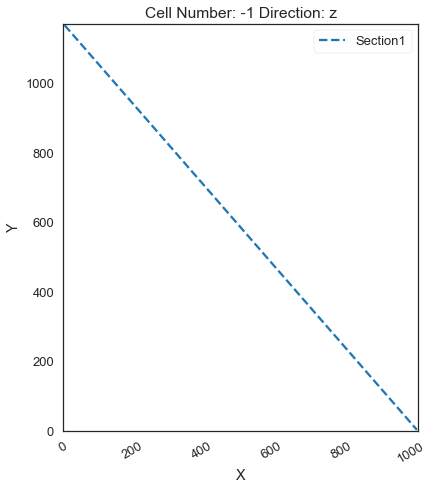
Defining Custom Section#
[31]:
custom_section = gpd.read_file(file_path + 'customsection26.shp')
custom_section_dict = gg.utils.to_section_dict(custom_section, section_column='name')
geo_model.set_section_grid(custom_section_dict)
Active grids: ['regular' 'topography' 'sections']
[31]:
| start | stop | resolution | dist | |
|---|---|---|---|---|
| Section1 | [3.685512376796794, 1168.3245583161138] | [1018.3144876418132, 2.95070672600923] | [100, 80] | 1545.18 |
[32]:
gp.plot.plot_section_traces(geo_model)
[32]:
<gempy.plot.visualization_2d.Plot2D at 0x1f10c056a90>
Plotting Input Data#
[33]:
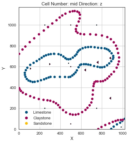
gp.plot_2d(geo_model, direction='z', show_lith=False, show_boundaries=False)
plt.grid()
[34]:
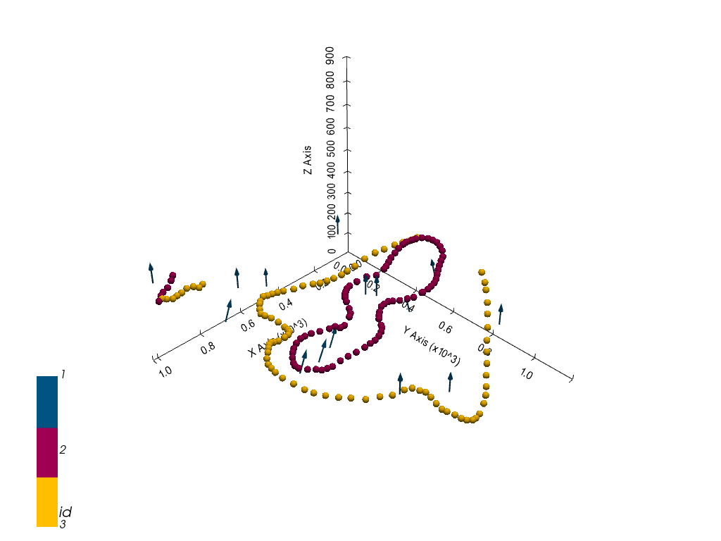
gp.plot_3d(geo_model, image=False, plotter_type='basic', notebook=True)
[34]:
<gempy.plot.vista.GemPyToVista at 0x1f107c86250>
Setting the Interpolator#
[35]:
gp.set_interpolator(geo_model,
                    compile_theano=True,
                    theano_optimizer='fast_compile',
                    verbose=[],
                    update_kriging = False
                    )
Compiling theano function...
Level of Optimization:  fast_compile
Device:  cpu
Precision:  float64
Number of faults:  0
Compilation Done!
Kriging values:
                   values
range            1796.68
$C_o$           76858.76
drift equations   [3, 3]
[35]:
<gempy.core.interpolator.InterpolatorModel at 0x1f10600b7c0>
Computing Model#
[36]:
sol = gp.compute_model(geo_model, compute_mesh=True)
Plotting Cross Sections#
[37]:
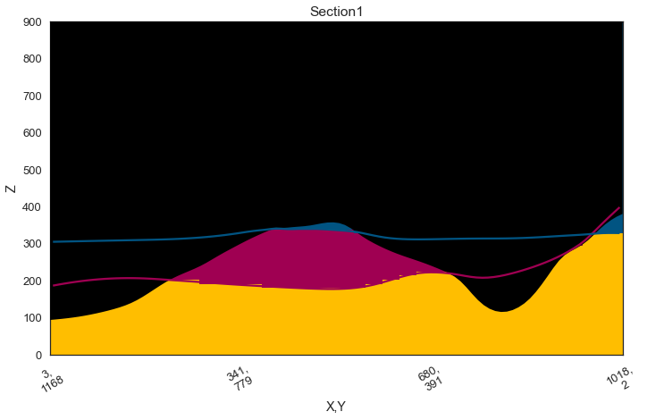
gp.plot_2d(geo_model, section_names=['Section1'], show_topography=True, show_data=False)
[37]:
<gempy.plot.visualization_2d.Plot2D at 0x1f108e93040>
[38]:
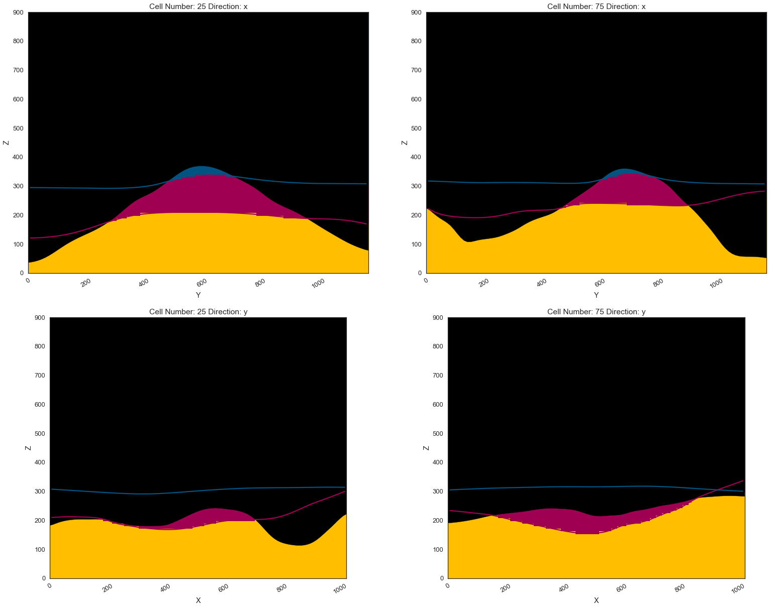
gp.plot_2d(geo_model, direction=['x', 'x', 'y', 'y'], cell_number=[25,75,25,75], show_topography=True, show_data=False)
[38]:
<gempy.plot.visualization_2d.Plot2D at 0x1f108ff1c70>
Plotting 3D Model#
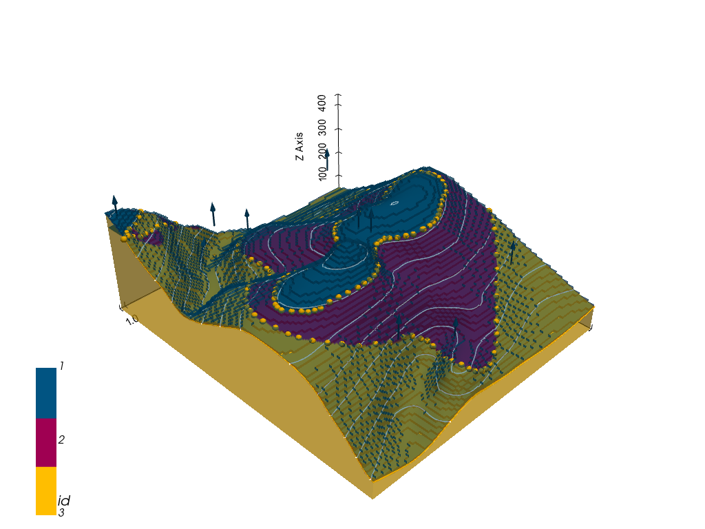
[39]:
gpv = gp.plot_3d(geo_model, image=False, show_topography=True,
                 plotter_type='basic', notebook=True, show_lith=True)
[ ]: