
Example 3 - Planar Dipping Layers
Contents
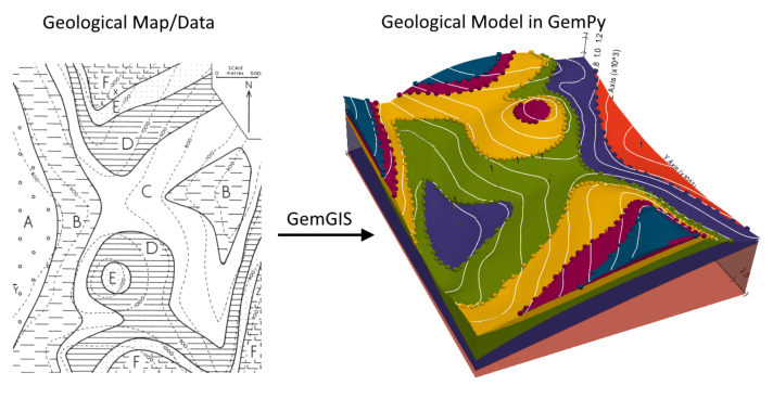
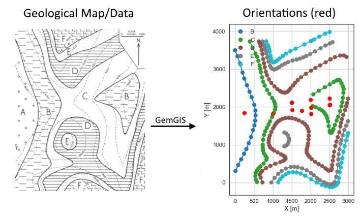
Example 3 - Planar Dipping Layers#
This example will show how to convert the geological map below using GemGIS to a GemPy model. This example is based on digitized data. The area is 3000 m wide (W-E extent) and 3740 m high (N-S extent). The vertical model extent varies between 200 m and 1200 m. The model represents several planar stratigraphic units (blue to purple) dipping towards the east above an unspecified basement (light red). The map has been georeferenced with QGIS. The stratigraphic boundaries were digitized in
QGIS. Strikes lines were digitized in QGIS as well and will be used to calculate orientations for the GemPy model. The contour lines were also digitized and will be interpolated with GemGIS to create a topography for the model.
Map Source: An Introduction to Geological Structures and Maps by G.M. Bennison
[1]:
import matplotlib.pyplot as plt
import matplotlib.image as mpimg
img = mpimg.imread('../images/cover_example03.png')
plt.figure(figsize=(10, 10))
imgplot = plt.imshow(img)
plt.axis('off')
plt.tight_layout()
Licensing#
Computational Geosciences and Reservoir Engineering, RWTH Aachen University, Authors: Alexander Juestel. For more information contact: alexander.juestel(at)rwth-aachen.de
This work is licensed under a Creative Commons Attribution 4.0 International License (http://creativecommons.org/licenses/by/4.0/)
Import GemGIS#
If you have installed GemGIS via pip or conda, you can import GemGIS like any other package. If you have downloaded the repository, append the path to the directory where the GemGIS repository is stored and then import GemGIS.
[2]:
import warnings
warnings.filterwarnings("ignore")
import gemgis as gg
Importing Libraries and loading Data#
All remaining packages can be loaded in order to prepare the data and to construct the model. The example data is downloaded from an external server using pooch. It will be stored in a data folder in the same directory where this notebook is stored.
[3]:
import geopandas as gpd
import rasterio
[4]:
file_path = 'data/example03/'
gg.download_gemgis_data.download_tutorial_data(filename="example03_planar_dipping_layers.zip", dirpath=file_path)
Downloading file 'example03_planar_dipping_layers.zip' from 'https://rwth-aachen.sciebo.de/s/AfXRsZywYDbUF34/download?path=%2Fexample03_planar_dipping_layers.zip' to 'C:\Users\ale93371\Documents\gemgis\docs\getting_started\example\data\example03'.
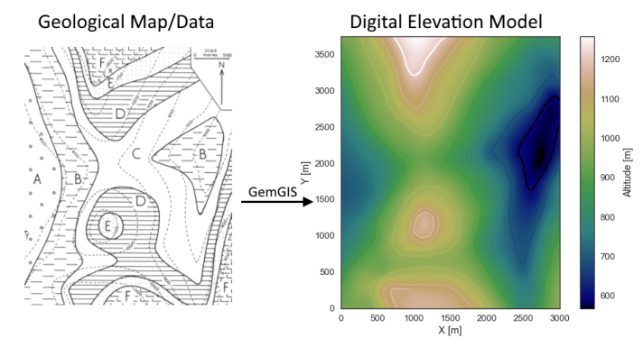
Creating Digital Elevation Model from Contour Lines#
The digital elevation model (DEM) will be created by interpolating contour lines digitized from the georeferenced map using the SciPy Radial Basis Function interpolation wrapped in GemGIS. The respective function used for that is gg.vector.interpolate_raster().
[5]:
import matplotlib.pyplot as plt
import matplotlib.image as mpimg
img = mpimg.imread('../images/dem_example03.png')
plt.figure(figsize=(10, 10))
imgplot = plt.imshow(img)
plt.axis('off')
plt.tight_layout()
[6]:
topo = gpd.read_file(file_path + 'topo3.shp')
topo.head()
[6]:
| id | Z | geometry | |
|---|---|---|---|
| 0 | None | 800 | LINESTRING (6.948 674.298, 97.151 781.847, 168... |
| 1 | None | 900 | LINESTRING (10.418 291.517, 78.648 414.099, 12... |
| 2 | None | 1100 | LINESTRING (978.357 1207.417, 1009.581 1271.02... |
| 3 | None | 1000 | LINESTRING (834.959 1363.536, 882.373 1447.956... |
| 4 | None | 1100 | LINESTRING (1778.613 2.407, 1712.696 100.704, ... |
Interpolating the contour lines#
[7]:
topo_raster = gg.vector.interpolate_raster(gdf=topo, value='Z', method='rbf', res=50)
Plotting the raster#
[8]:
import matplotlib.pyplot as plt

fix, ax = plt.subplots(1, figsize=(10, 10))
topo.plot(ax=ax, aspect='equal', column='Z', cmap='gist_earth')
im = plt.imshow(topo_raster, origin='lower', extent=[0, 3000, 0, 3740], cmap='gist_earth')
cbar = plt.colorbar(im)
cbar.set_label('Altitude [m]')
ax.set_xlabel('X [m]')
ax.set_ylabel('Y [m]')
ax.set_xlim(0, 3000)
ax.set_ylim(0, 3740)
[8]:
(0.0, 3740.0)
Saving the raster to disc#
After the interpolation of the contour lines, the raster is saved to disc using gg.raster.save_as_tiff(). The function will not be executed as a raster is already provided with the example data.
Opening Raster#
The previously computed and saved raster can now be opened using rasterio.
[9]:
topo_raster = rasterio.open(file_path + 'raster3.tif')
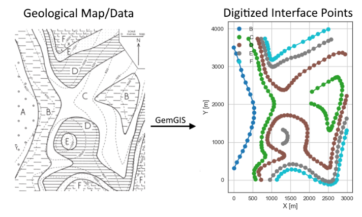
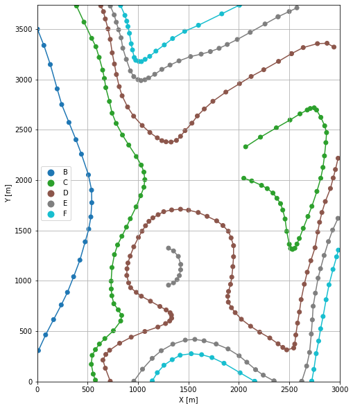
Interface Points of stratigraphic boundaries#
The interface points will be extracted from LineStrings digitized from the georeferenced map using QGIS. It is important to provide a formation name for each layer boundary. The vertical position of the interface point will be extracted from the digital elevation model using the GemGIS function gg.vector.extract_xyz(). The resulting GeoDataFrame now contains single points including the information about the respective formation.
[10]:
import matplotlib.pyplot as plt
import matplotlib.image as mpimg
img = mpimg.imread('../images/interfaces_example03.png')
plt.figure(figsize=(10, 10))
imgplot = plt.imshow(img)
plt.axis('off')
plt.tight_layout()
[11]:
interfaces = gpd.read_file(file_path + 'interfaces3.shp')
interfaces.head()
[11]:
| id | formation | geometry | |
|---|---|---|---|
| 0 | None | B | LINESTRING (2.323 3499.479, 65.927 3338.734, 1... |
| 1 | None | C | LINESTRING (389.730 3730.767, 463.742 3570.022... |
| 2 | None | C | LINESTRING (2067.723 2331.475, 2214.591 2427.4... |
| 3 | None | D | LINESTRING (2522.204 3256.627, 2393.839 3180.3... |
| 4 | None | E | LINESTRING (2389.213 3623.218, 2259.692 3551.5... |
Extracting Z coordinate from Digital Elevation Model#
[12]:
interfaces_coords = gg.vector.extract_xyz(gdf=interfaces, dem=topo_raster)
interfaces_coords = interfaces_coords.sort_values(by='formation', ascending=False)
interfaces_coords
[12]:
| formation | geometry | X | Y | Z | |
|---|---|---|---|---|---|
| 169 | F | POINT (932.100 3354.924) | 932.10 | 3354.92 | 1214.19 |
| 170 | F | POINT (914.753 3459.004) | 914.75 | 3459.00 | 1213.03 |
| 181 | F | POINT (1630.589 267.231) | 1630.59 | 267.23 | 1085.09 |
| 180 | F | POINT (1527.666 276.483) | 1527.67 | 276.48 | 1101.00 |
| 179 | F | POINT (1417.804 261.449) | 1417.80 | 261.45 | 1118.56 |
| ... | ... | ... | ... | ... | ... |
| 17 | B | POINT (238.236 761.031) | 238.24 | 761.03 | 854.53 |
| 18 | B | POINT (161.911 615.320) | 161.91 | 615.32 | 870.34 |
| 19 | B | POINT (83.273 463.826) | 83.27 | 463.83 | 886.53 |
| 20 | B | POINT (11.574 307.707) | 11.57 | 307.71 | 895.69 |
| 0 | B | POINT (2.323 3499.479) | 2.32 | 3499.48 | 898.42 |
339 rows × 5 columns
Plotting the Interface Points#
[13]:
fig, ax = plt.subplots(1, figsize=(10, 10))

interfaces.plot(ax=ax, column='formation', legend=True, aspect='equal')
interfaces_coords.plot(ax=ax, column='formation', legend=True, aspect='equal')
plt.grid()
ax.set_xlabel('X [m]')
ax.set_ylabel('Y [m]')
ax.set_xlim(0, 3000)
ax.set_ylim(0, 3740)
[13]:
(0.0, 3740.0)
Orientations from Strike Lines#
Strike lines connect outcropping stratigraphic boundaries (interfaces) of the same altitude. In other words: the intersections between topographic contours and stratigraphic boundaries at the surface. The height difference and the horizontal difference between two digitized lines is used to calculate the dip and azimuth and hence an orientation that is necessary for GemPy. In order to calculate the orientations, each set of strikes lines/LineStrings for one formation must be given an id
number next to the altitude of the strike line. The id field is already predefined in QGIS. The strike line with the lowest altitude gets the id number 1, the strike line with the highest altitude the the number according to the number of digitized strike lines. It is currently recommended to use one set of strike lines for each structural element of one formation as illustrated.
[14]:
import matplotlib.pyplot as plt
import matplotlib.image as mpimg
img = mpimg.imread('../images/orientations_example03.png')
plt.figure(figsize=(10, 10))
imgplot = plt.imshow(img)
plt.axis('off')
plt.tight_layout()
[15]:
strikes = gpd.read_file(file_path + 'strikes3.shp')
strikes
[15]:
| id | formation | Z | geometry | |
|---|---|---|---|---|
| 0 | 2 | C | 700 | LINESTRING (2236.563 2441.337, 2244.658 1935.973) |
| 1 | 1 | C | 600 | LINESTRING (2752.335 2715.413, 2750.022 1809.921) |
| 2 | 2 | D | 800 | LINESTRING (2242.924 3096.460, 2290.338 441.276) |
| 3 | 3 | D | 900 | LINESTRING (1739.873 2780.752, 1758.376 1605.810) |
| 4 | 4 | D | 1000 | LINESTRING (1236.822 2394.501, 1239.134 1677.509) |
| 5 | 4 | E | 1100 | LINESTRING (1245.495 953.000, 1236.243 3100.507) |
| 6 | 3 | E | 1000 | LINESTRING (1749.124 3284.381, 1790.756 364.372) |
| 7 | 2 | E | 900 | LINESTRING (2242.345 63.698, 2259.692 3551.519) |
| 8 | 1 | F | 1000 | LINESTRING (2012.214 86.827, 2005.275 3738.862) |
| 9 | 2 | F | 1100 | LINESTRING (1534.026 272.435, 1499.911 3496.010) |
| 10 | 1 | A | 800 | LINESTRING (486.292 2124.473, 495.544 1456.051) |
| 11 | 2 | A | 900 | LINESTRING (2.323 3499.479, 11.574 307.707) |
| 12 | 5 | C | 1000 | LINESTRING (736.009 2693.445, 761.729 511.476) |
| 13 | 1 | B | 800 | LINESTRING (489.213 2109.525, 496.562 1470.183) |
| 14 | 2 | B | 900 | LINESTRING (2.323 3499.479, 11.574 307.707) |
| 15 | 1 | D | 700 | LINESTRING (2752.631 1310.960, 2747.732 3388.209) |
| 16 | 1 | E | 800 | LINESTRING (2745.282 835.740, 2750.181 3753.197) |
| 17 | 3 | C | 800 | LINESTRING (1759.324 1605.522, 1739.727 2783.774) |
| 18 | 4 | C | 900 | LINESTRING (1238.786 1676.560, 1237.562 2396.739) |
Calculate Orientations for each formation#
[16]:
orientations_b = gg.vector.calculate_orientations_from_strike_lines(gdf=strikes[strikes['formation'] == 'B'].sort_values(by='id', ascending=True).reset_index())
orientations_b
[16]:
| dip | azimuth | Z | geometry | polarity | formation | X | Y | |
|---|---|---|---|---|---|---|---|---|
| 0 | 11.70 | 89.81 | 850.00 | POINT (249.918 1846.723) | 1.00 | B | 249.92 | 1846.72 |
[17]:
orientations_c = gg.vector.calculate_orientations_from_strike_lines(gdf=strikes[strikes['formation'] == 'C'].sort_values(by='id', ascending=True).reset_index())
orientations_c
[17]:
| dip | azimuth | Z | geometry | polarity | formation | X | Y | |
|---|---|---|---|---|---|---|---|---|
| 0 | 11.19 | 89.89 | 650.00 | POINT (2495.895 2225.661) | 1.00 | C | 2495.89 | 2225.66 |
| 1 | 11.52 | 89.05 | 750.00 | POINT (1995.068 2191.652) | 1.00 | C | 1995.07 | 2191.65 |
| 2 | 11.12 | 89.28 | 850.00 | POINT (1493.850 2115.649) | 1.00 | C | 1493.85 | 2115.65 |
| 3 | 11.52 | 89.38 | 950.00 | POINT (993.522 1819.555) | 1.00 | C | 993.52 | 1819.56 |
[18]:
orientations_d = gg.vector.calculate_orientations_from_strike_lines(gdf=strikes[strikes['formation'] == 'D'].sort_values(by='id', ascending=True).reset_index())
orientations_d
[18]:
| dip | azimuth | Z | geometry | polarity | formation | X | Y | |
|---|---|---|---|---|---|---|---|---|
| 0 | 11.82 | 89.31 | 750.00 | POINT (2508.406 2059.226) | 1.00 | D | 2508.41 | 2059.23 |
| 1 | 11.12 | 89.00 | 850.00 | POINT (2007.877 1981.074) | 1.00 | D | 2007.88 | 1981.07 |
| 2 | 11.11 | 89.29 | 950.00 | POINT (1493.551 2114.643) | 1.00 | D | 1493.55 | 2114.64 |
[19]:
orientations_e = gg.vector.calculate_orientations_from_strike_lines(gdf=strikes[strikes['formation'] == 'E'].sort_values(by='Z', ascending=True).reset_index())
orientations_e
[19]:
| dip | azimuth | Z | geometry | polarity | formation | X | Y | |
|---|---|---|---|---|---|---|---|---|
| 0 | 11.53 | 90.21 | 850.00 | POINT (2499.375 2051.039) | 1.00 | E | 2499.38 | 2051.04 |
| 1 | 12.45 | 89.83 | 950.00 | POINT (2010.479 1815.993) | 1.00 | E | 2010.48 | 1815.99 |
| 2 | 10.98 | 89.38 | 1050.00 | POINT (1505.405 1925.565) | 1.00 | E | 1505.40 | 1925.57 |
[20]:
orientations_f = gg.vector.calculate_orientations_from_strike_lines(gdf=strikes[strikes['formation'] == 'F'].sort_values(by='id', ascending=True).reset_index())
orientations_f
[20]:
| dip | azimuth | Z | geometry | polarity | formation | X | Y | |
|---|---|---|---|---|---|---|---|---|
| 0 | 11.82 | 89.67 | 1050.00 | POINT (1762.857 1898.533) | 1.00 | F | 1762.86 | 1898.53 |
Merging Orientations#
[21]:
import pandas as pd
orientations = pd.concat([orientations_b, orientations_c, orientations_d, orientations_e, orientations_f])
orientations = orientations[orientations['formation'].isin(['F', 'E', 'D', 'C', 'B'])].reset_index()
orientations
[21]:
| index | dip | azimuth | Z | geometry | polarity | formation | X | Y | |
|---|---|---|---|---|---|---|---|---|---|
| 0 | 0 | 11.70 | 89.81 | 850.00 | POINT (249.918 1846.723) | 1.00 | B | 249.92 | 1846.72 |
| 1 | 0 | 11.19 | 89.89 | 650.00 | POINT (2495.895 2225.661) | 1.00 | C | 2495.89 | 2225.66 |
| 2 | 1 | 11.52 | 89.05 | 750.00 | POINT (1995.068 2191.652) | 1.00 | C | 1995.07 | 2191.65 |
| 3 | 2 | 11.12 | 89.28 | 850.00 | POINT (1493.850 2115.649) | 1.00 | C | 1493.85 | 2115.65 |
| 4 | 3 | 11.52 | 89.38 | 950.00 | POINT (993.522 1819.555) | 1.00 | C | 993.52 | 1819.56 |
| 5 | 0 | 11.82 | 89.31 | 750.00 | POINT (2508.406 2059.226) | 1.00 | D | 2508.41 | 2059.23 |
| 6 | 1 | 11.12 | 89.00 | 850.00 | POINT (2007.877 1981.074) | 1.00 | D | 2007.88 | 1981.07 |
| 7 | 2 | 11.11 | 89.29 | 950.00 | POINT (1493.551 2114.643) | 1.00 | D | 1493.55 | 2114.64 |
| 8 | 0 | 11.53 | 90.21 | 850.00 | POINT (2499.375 2051.039) | 1.00 | E | 2499.38 | 2051.04 |
| 9 | 1 | 12.45 | 89.83 | 950.00 | POINT (2010.479 1815.993) | 1.00 | E | 2010.48 | 1815.99 |
| 10 | 2 | 10.98 | 89.38 | 1050.00 | POINT (1505.405 1925.565) | 1.00 | E | 1505.40 | 1925.57 |
| 11 | 0 | 11.82 | 89.67 | 1050.00 | POINT (1762.857 1898.533) | 1.00 | F | 1762.86 | 1898.53 |
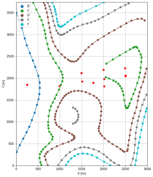
Plotting the Orientations#
[22]:
fig, ax = plt.subplots(1, figsize=(10, 10))

interfaces.plot(ax=ax, column='formation', legend=True, aspect='equal')
interfaces_coords.plot(ax=ax, column='formation', legend=True, aspect='equal')
orientations.plot(ax=ax, color='red', aspect='equal')
plt.grid()
ax.set_xlabel('X [m]')
ax.set_ylabel('Y [m]')
ax.set_xlim(0, 3000)
ax.set_ylim(0, 3740)
[22]:
(0.0, 3740.0)
GemPy Model Construction#
The structural geological model will be constructed using the GemPy package.
[23]:
import gempy as gp
WARNING (theano.configdefaults): g++ not available, if using conda: `conda install m2w64-toolchain`
WARNING (theano.configdefaults): g++ not detected ! Theano will be unable to execute optimized C-implementations (for both CPU and GPU) and will default to Python implementations. Performance will be severely degraded. To remove this warning, set Theano flags cxx to an empty string.
WARNING (theano.tensor.blas): Using NumPy C-API based implementation for BLAS functions.
Creating new Model#
[24]:
geo_model = gp.create_model('Model3')
geo_model
[24]:
Model3 2022-04-04 15:53
Initiate Data#
[25]:
gp.init_data(geo_model, [0, 3000, 0, 3740, 200, 1200], [100, 100, 100],
             surface_points_df=interfaces_coords[interfaces_coords['Z'] != 0],
             orientations_df=orientations,
             default_values=True)
Active grids: ['regular']
[25]:
Model3 2022-04-04 15:53
Model Surfaces#
[26]:
geo_model.surfaces
[26]:
| surface | series | order_surfaces | color | id | |
|---|---|---|---|---|---|
| 0 | F | Default series | 1 | #015482 | 1 |
| 1 | E | Default series | 2 | #9f0052 | 2 |
| 2 | D | Default series | 3 | #ffbe00 | 3 |
| 3 | C | Default series | 4 | #728f02 | 4 |
| 4 | B | Default series | 5 | #443988 | 5 |
Mapping the Stack to Surfaces#
[27]:
gp.map_stack_to_surfaces(geo_model,
                         {
                          'Strata1': ('F'),
                          'Strata2': ('E'),
                          'Strata3': ('D'),
                          'Strata4': ('C'),
                          'Strata5': ('B'),
                         },
                         remove_unused_series=True)
geo_model.add_surfaces('A')
[27]:
| surface | series | order_surfaces | color | id | |
|---|---|---|---|---|---|
| 0 | F | Strata1 | 1 | #015482 | 1 |
| 1 | E | Strata2 | 1 | #9f0052 | 2 |
| 2 | D | Strata3 | 1 | #ffbe00 | 3 |
| 3 | C | Strata4 | 1 | #728f02 | 4 |
| 4 | B | Strata5 | 1 | #443988 | 5 |
| 5 | A | Strata5 | 2 | #ff3f20 | 6 |
Showing the Number of Data Points#
[28]:
gg.utils.show_number_of_data_points(geo_model=geo_model)
[28]:
| surface | series | order_surfaces | color | id | No. of Interfaces | No. of Orientations | |
|---|---|---|---|---|---|---|---|
| 0 | F | Strata1 | 1 | #015482 | 1 | 45 | 1 |
| 1 | E | Strata2 | 1 | #9f0052 | 2 | 68 | 3 |
| 2 | D | Strata3 | 1 | #ffbe00 | 3 | 113 | 3 |
| 3 | C | Strata4 | 1 | #728f02 | 4 | 77 | 4 |
| 4 | B | Strata5 | 1 | #443988 | 5 | 21 | 1 |
| 5 | A | Strata5 | 2 | #ff3f20 | 6 | 0 | 0 |
Loading Digital Elevation Model#
[29]:
geo_model.set_topography(source='gdal', filepath=file_path + 'raster3.tif')
Cropped raster to geo_model.grid.extent.
depending on the size of the raster, this can take a while...
storing converted file...
Active grids: ['regular' 'topography']
[29]:
Grid Object. Values:
array([[  15.        ,   18.7       ,  205.        ],
       [  15.        ,   18.7       ,  215.        ],
       [  15.        ,   18.7       ,  225.        ],
       ...,
       [2992.5       , 3702.6       ,  833.75482178],
       [2992.5       , 3717.56      ,  838.74261475],
       [2992.5       , 3732.52      ,  843.78088379]])
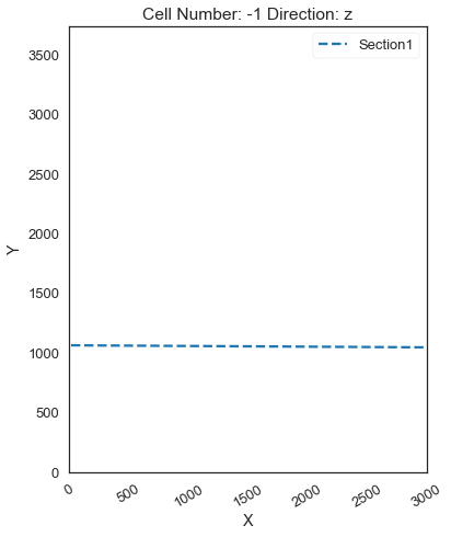
Defining Custom Section#
[30]:
custom_section = gpd.read_file(file_path + 'customsection3.shp')
custom_section_dict = gg.utils.to_section_dict(custom_section, section_column='name')
geo_model.set_section_grid(custom_section_dict)
Active grids: ['regular' 'topography' 'sections']
[30]:
| start | stop | resolution | dist | |
|---|---|---|---|---|
| Section1 | [15.217892876134727, 1063.5514258527073] | [2991.4655480049296, 1046.4043200206897] | [100, 80] | 2976.30 |
[31]:
gp.plot.plot_section_traces(geo_model)
[31]:
<gempy.plot.visualization_2d.Plot2D at 0x1d547775a90>
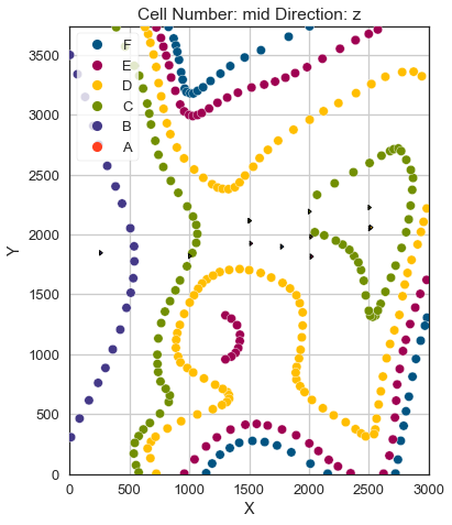
Plotting Input Data#
[32]:
gp.plot_2d(geo_model, direction='z', show_lith=False, show_boundaries=False)
plt.grid()
[33]:
gp.plot_3d(geo_model, image=False, plotter_type='basic', notebook=True)
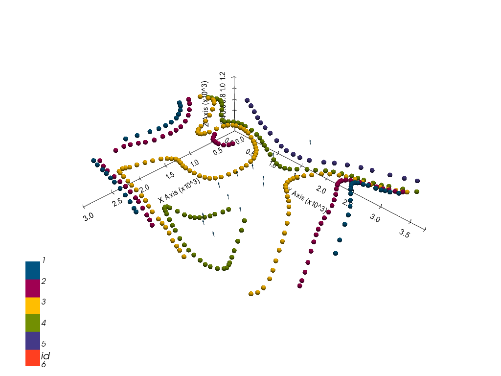
[33]:
<gempy.plot.vista.GemPyToVista at 0x1d5431d25e0>
Setting the Interpolator#
[34]:
gp.set_interpolator(geo_model,
                    compile_theano=True,
                    theano_optimizer='fast_compile',
                    verbose=[],
                    update_kriging=False
                    )
Compiling theano function...
Level of Optimization:  fast_compile
Device:  cpu
Precision:  float64
Number of faults:  0
Compilation Done!
Kriging values:
                           values
range                    4897.71
$C_o$                  571133.33
drift equations  [3, 3, 3, 3, 3]
[34]:
<gempy.core.interpolator.InterpolatorModel at 0x1d541724ac0>
Computing Model#
[35]:
sol = gp.compute_model(geo_model, compute_mesh=True)
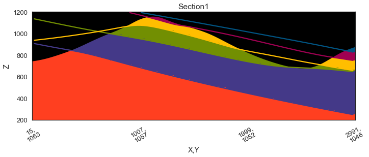
Plotting Cross Sections#
[36]:
gp.plot_2d(geo_model, section_names=['Section1'], show_topography=True, show_data=False)
[36]:
<gempy.plot.visualization_2d.Plot2D at 0x1d545715c70>
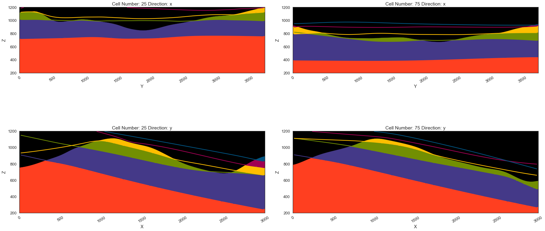
[37]:
gp.plot_2d(geo_model, direction=['x', 'x', 'y', 'y'], cell_number=[25, 75, 25, 75], show_topography=True, show_data=False)
[37]:
<gempy.plot.visualization_2d.Plot2D at 0x1d54868da30>
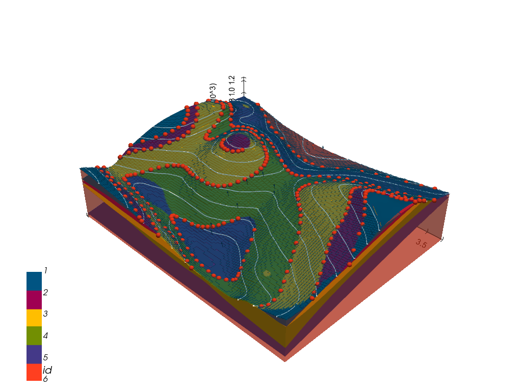
Plotting 3D Model#
[38]:
gpv = gp.plot_3d(geo_model, image=False, show_topography=True,
                 plotter_type='basic', notebook=True, show_lith=True)
[ ]: