50 Parsing Leapfrog Wells

Leapfrog provides well data in the form of several CSV files. These include a collar file, a survey file, a litho file and an assay file. With GemGIS it is now possible to read in these wells and visualize them.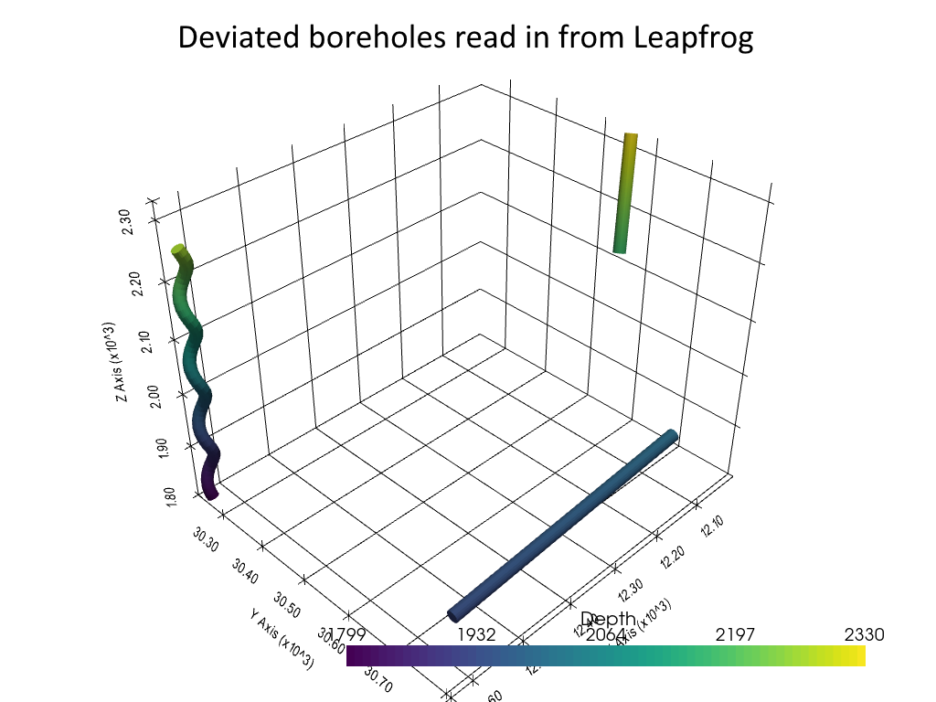

Set File Paths and download Tutorial Data

If you downloaded the latest GemGIS version from the Github repository, append the path so that the package can be imported successfully. Otherwise, it is recommended to install GemGIS via pip install gemgis and import GemGIS using import gemgis as gg. In addition, the file path to the folder where the data is being stored is set. The tutorial data is downloaded using Pooch (https://www.fatiando.org/pooch/latest/index.html) and stored in the specified folder. Use pip install pooch if Pooch is not installed on your system yet.

import gemgis as gg

file_path ='data/50_parsing_leapfrog_wells/'

WARNING (theano.configdefaults): g++ not available, if using conda: `conda install m2w64-toolchain`
C:\Users\ale93371\Anaconda3\envs\test_gempy\lib\site-packages\theano\configdefaults.py:560: UserWarning: DeprecationWarning: there is no c++ compiler.This is deprecated and with Theano 0.11 a c++ compiler will be mandatory
  warnings.warn("DeprecationWarning: there is no c++ compiler."
WARNING (theano.configdefaults): g++ not detected ! Theano will be unable to execute optimized C-implementations (for both CPU and GPU) and will default to Python implementations. Performance will be severely degraded. To remove this warning, set Theano flags cxx to an empty string.
WARNING (theano.tensor.blas): Using NumPy C-API based implementation for BLAS functions.

gg.download_gemgis_data.download_tutorial_data(filename="50_parsing_leapfrog_wells.zip", dirpath=file_path)

Downloading file '50_parsing_leapfrog_wells.zip' from 'https://rwth-aachen.sciebo.de/s/AfXRsZywYDbUF34/download?path=%2F50_parsing_leapfrog_wells.zip' to 'C:\Users\ale93371\Documents\gemgis\docs\getting_started\tutorial\data\50_parsing_leapfrog_wells'.

Loading Data

The Leapfrog well data is read in as Pandas DataFrames.

import pandas as pd

litho = pd.read_csv(file_path+'litho.csv')
litho.head()

WARNING (theano.configdefaults): g++ not available, if using conda: `conda install m2w64-toolchain`
C:\Users\ale93371\Anaconda3\envs\test_gempy\lib\site-packages\theano\configdefaults.py:560: UserWarning: DeprecationWarning: there is no c++ compiler.This is deprecated and with Theano 0.11 a c++ compiler will be mandatory
  warnings.warn("DeprecationWarning: there is no c++ compiler."
WARNING (theano.configdefaults): g++ not detected ! Theano will be unable to execute optimized C-implementations (for both CPU and GPU) and will default to Python implementations. Performance will be severely degraded. To remove this warning, set Theano flags cxx to an empty string.
WARNING (theano.tensor.blas): Using NumPy C-API based implementation for BLAS functions.

	holeid	from	to	Geology
0	UG_034	0.00	24.46	Conglomerate
1	UG_034	24.46	44.01	Arkoses
2	UG_034	44.01	122.29	Quartzitic sandstones
3	UG_034	122.29	140.70	Quartzites
4	UG_034	140.70	180.00	Lower Black shales

collar = pd.read_csv(file_path+'collar.csv', delimiter=';')
collar

	holeid	x	y	z	maxdepth	comment
0	UG_034	12172.83	30799.71	1977.71	180	underground DH, upwards
1	RWTHO_006	12628.76	30259.13	2259.59	450	inclined
2	SonicS_006	12012.68	30557.53	2325.53	500	lift

survey = pd.read_csv(file_path+'survey.csv')
survey.head()

	holeid	depth	dip	azimuth
0	UG_034	0	-65.00	20
1	UG_034	180	-65.00	20
2	RWTHO_006	0	55.00	308
3	RWTHO_006	450	55.00	308
4	SonicS_006	0	90.00	20

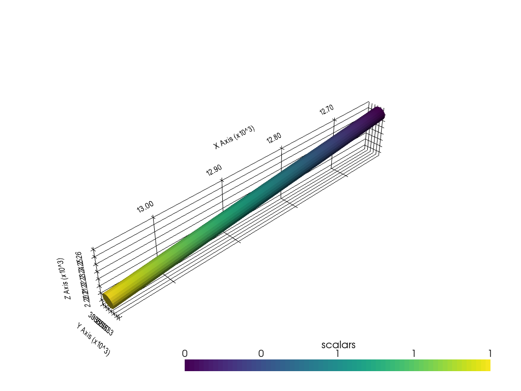
Plotting the first well

The first well to be plotted is well SonicS_006.

survey006 = survey[survey['holeid']=='SonicS_006']
survey006 = survey006.reset_index().drop('index', axis=1)
survey006.head()

	holeid	depth	dip	azimuth
0	SonicS_006	0	90.00	20
1	SonicS_006	10	89.50	20
2	SonicS_006	20	89.00	20
3	SonicS_006	30	88.50	20
4	SonicS_006	40	88.00	20

Getting the coordinates of the well at the surface.

x0 = collar[['x', 'y', 'z']].loc[2].values
x0

array([12012.68053 , 30557.53476 ,  2325.532416])

Creating the DataFrame from which the well paths are created.

df_survey = gg.visualization.create_deviated_borehole_df(df_survey=survey006, position=x0)
df_survey.head()

	holeid	depth	dip	azimuth	depth_bottom	vector	segment_length	X	Y	Z	points
0	SonicS_006	0	90.00	20	10.00	[[0.36482400173640905], [-0.18285080511417406]...	-10	12012.68	30557.53	2325.53	[12012.68053, 30557.534760000002, 2325.532416]
1	SonicS_006	0	90.00	20	10.00	[[0.36482400173640905], [-0.18285080511417406]...	-10	12009.03	30559.36	2316.40	[12009.032289982635, 30559.363268051144, 2316....
2	SonicS_006	10	89.50	20	20.00	[[0.4078265278090107], [0.014439265532404447],...	-10	12004.95	30559.22	2307.27	[12004.954024704546, 30559.21887539582, 2307.2...
3	SonicS_006	20	89.00	20	30.00	[[0.3509788964265648], [0.2081941003896598], [...	-10	12001.44	30557.14	2298.14	[12001.44423574028, 30557.136934391925, 2298.1...
4	SonicS_006	30	88.50	20	40.00	[[0.2081993903819504], [0.3509757584484337], [...	-10	11999.36	30553.63	2289.01	[11999.362241836461, 30553.62717680744, 2289.0...

Creating lines from DataFrame.

lines = gg.visualization.create_lines_from_points(df=df_survey)
lines

PolyData	Information
N Cells	52
N Points	51
X Bounds	1.200e+04, 1.202e+04
Y Bounds	3.054e+04, 3.056e+04
Z Bounds	1.869e+03, 2.326e+03
N Arrays	0

Creating tubes from lines.

tubes = gg.visualization.create_borehole_tube(df=df_survey, line=lines, radius=10)
tubes

Header	Data Arrays
PolyData Information N Cells 22 N Points 1060 X Bounds 1.199e+04, 1.203e+04 Y Bounds 3.053e+04, 3.057e+04 Z Bounds 1.865e+03, 2.330e+03 N Arrays 3	Name Field Type N Comp Min Max scalars Points int32 1 0.000e+00 5.000e+01 TubeNormals Points float32 3 -9.996e-01 9.996e-01 Depth Points float64 1 1.865e+03 2.330e+03

Plotting the well.

import pyvista as pv

sargs = dict(fmt="%.0f", color='black')

p = pv.Plotter(notebook=True)

# Adding DEM
p.add_mesh(tubes, scalars='Depth', scalar_bar_args=sargs)


p.set_background('white')
p.show_grid(color='black')
p.set_scale(1,1,1)
p.show()

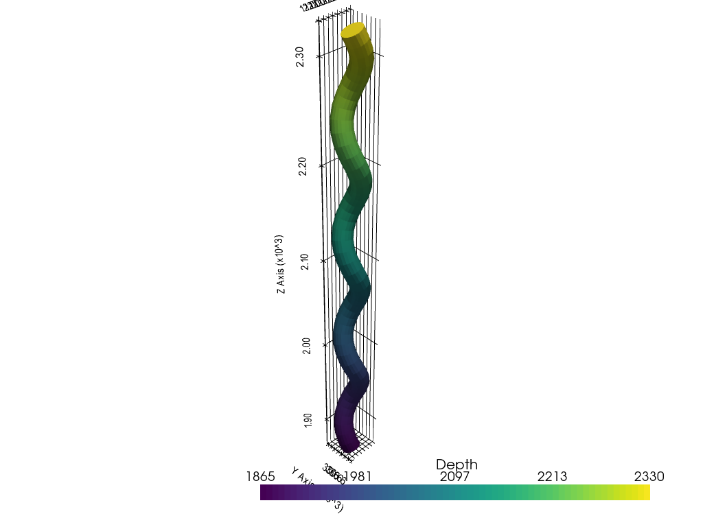
Plotting the second well

The second well that will be plotted is RWTHO_006.

surveyrwth = survey[survey['holeid']=='RWTHO_006']
surveyrwth = surveyrwth.reset_index().drop('index', axis=1)
surveyrwth.head()

	holeid	depth	dip	azimuth
0	RWTHO_006	0	55.00	308
1	RWTHO_006	450	55.00	308

Getting the coordinates of the well at the surface.

x0 = collar[['x', 'y', 'z']].loc[1].values
x0

array([12628.75598, 30259.12988,  2259.59034])

Creating the DataFrame from which the well paths are created.

df_survey = gg.visualization.create_deviated_borehole_df(df_survey=surveyrwth, position=x0)
df_survey

	holeid	depth	dip	azimuth	depth_bottom	vector	segment_length	X	Y	Z	points
0	RWTHO_006	0	55.00	308	450.00	[[-0.992088794420255], [0.021957082623147627],...	-450	12628.76	30259.13	2259.59	[12628.75598, 30259.12988, 2259.5903399999997]
1	RWTHO_006	0	55.00	308	450.00	[[-0.992088794420255], [0.021957082623147627],...	-450	13075.20	30249.25	2203.97	[13075.195937489114, 30249.249192819585, 2203....

Creating lines from DataFrame.

lines = gg.visualization.create_lines_from_points(df=df_survey)
lines

PolyData	Information
N Cells	3
N Points	2
X Bounds	1.263e+04, 1.308e+04
Y Bounds	3.025e+04, 3.026e+04
Z Bounds	2.204e+03, 2.260e+03
N Arrays	0

Creating tubes from lines.

tubes = gg.visualization.create_borehole_tube(df=df_survey, line=lines, radius=10)
tubes

Header	Data Arrays
PolyData Information N Cells 22 N Points 80 X Bounds 1.263e+04, 1.308e+04 Y Bounds 3.024e+04, 3.027e+04 Z Bounds 2.194e+03, 2.270e+03 N Arrays 3	Name Field Type N Comp Min Max scalars Points int32 1 0.000e+00 1.000e+00 TubeNormals Points float32 3 -9.998e-01 9.998e-01 Depth Points float64 1 2.194e+03 2.270e+03

Plotting the well.

import pyvista as pv

sargs = dict(fmt="%.0f", color='black')

p = pv.Plotter(notebook=True)

# Adding DEM
p.add_mesh(tubes, scalar_bar_args=sargs)


p.set_background('white')
p.show_grid(color='black')
p.set_scale(1,1,1)
p.show()

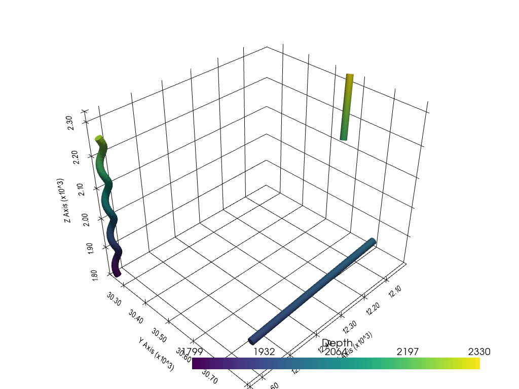
Creating tubes for all wells

All tubes for all wells can be created with the function create_deviated_boreholes_3d(..).

tubes, df_groups = gg.visualization.create_deviated_boreholes_3d(df_collar=collar,
                                                                 df_survey=survey,
                                                                 min_length=10,
                                                                 collar_depth='maxdepth',
                                                                 survey_depth='depth',
                                                                 index='holeid')
tubes

Information	Blocks
MultiBlock Values N Blocks 3 X Bounds 12003.268, 12641.589 Y Bounds 30234.730, 30809.708 Z Bounds 1799.074, 2329.613	Index Name Type 0 Block-00 PolyData 1 Block-01 PolyData 2 Block-02 PolyData

import pyvista as pv

sargs = dict(fmt="%.0f", color='black')

p = pv.Plotter(notebook=True)

# Adding DEM
p.add_mesh(tubes, scalars='Depth', scalar_bar_args=sargs)


p.set_background('white')
p.show_grid(color='black')
p.set_scale(1,1,1)
p.show()