59 Visualizing DoubletCalc Results
Contents
59 Visualizing DoubletCalc Results#
This notebook illustrates how to create the output plots provided by DoubletCalc with matplotlib.
Importing Libraries#
[1]:
import pandas as pd
import numpy as np
import matplotlib.pyplot as plt
Reading DoubletCalc Results CSV File#
[2]:
data = pd.read_csv('data/export_output.csv',
                   skiprows = 2,
                   delimiter = ',',
                   encoding = "ISO-8859-1",
                   skipfooter = 1)
data
C:\Users\ale93371\AppData\Local\Temp\ipykernel_15364\1359617900.py:1: ParserWarning: Falling back to the 'python' engine because the 'c' engine does not support skipfooter; you can avoid this warning by specifying engine='python'.
  data = pd.read_csv('data/export_output.csv',
[2]:
| iS | aquifer permeability (mD) | aquifer gross thickness (m) | aquifer net to gross (-) | aquifer top at injector (m TVD) | aquifer top at producer (m TVD) | aquifer water salinity (ppm) | aquifer kH net (Dm) | mass flow (kg/s) | delta T (°C) | heat capacity (kJ/(kg*K)) | av. production density (kg/m³) | required pump power (kW) | pump volume flow (m³/h) | geothermal power (MW) | COP (kW/kW) | |
|---|---|---|---|---|---|---|---|---|---|---|---|---|---|---|---|---|
| 0 | 1 | 254.29453 | 98.67665 | 0.809259 | 2458.3457 | 2457.9678 | 0.119523 | 20.306683 | 40.136295 | 49.975120 | 3664.4312 | 1057.3365 | 248.91680 | 136.65536 | 7.350175 | 29.528645 |
| 1 | 2 | 232.21005 | 101.61317 | 0.787313 | 2643.6982 | 2521.1965 | 0.123078 | 18.577118 | 37.513557 | 51.644176 | 3651.1710 | 1058.8849 | 232.31094 | 127.53875 | 7.073621 | 30.448938 |
| 2 | 3 | 347.02588 | 110.62248 | 0.783280 | 2322.7173 | 2336.0005 | 0.102066 | 30.069246 | 51.665833 | 47.223145 | 3733.5127 | 1046.2684 | 323.81015 | 177.77185 | 9.109110 | 28.131021 |
| 3 | 4 | 416.37143 | 110.71101 | 0.793836 | 2409.1120 | 2465.4832 | 0.126697 | 36.593388 | 57.302696 | 51.169163 | 3636.7332 | 1062.0903 | 353.78850 | 194.22997 | 10.663378 | 30.140543 |
| 4 | 5 | 385.43112 | 106.67485 | 0.803228 | 2553.3394 | 2534.5093 | 0.123331 | 33.025370 | 54.664562 | 53.064050 | 3650.8708 | 1058.3341 | 338.69850 | 185.94554 | 10.590165 | 31.267237 |
| ... | ... | ... | ... | ... | ... | ... | ... | ... | ... | ... | ... | ... | ... | ... | ... | ... |
| 995 | 996 | 208.79338 | 107.78278 | 0.796793 | 2371.8330 | 2634.3254 | 0.116407 | 17.931303 | 38.144660 | 55.109097 | 3679.4836 | 1051.8035 | 237.80956 | 130.55750 | 7.734708 | 32.524796 |
| 996 | 997 | 335.04092 | 107.57787 | 0.803419 | 2431.6885 | 2622.8328 | 0.123286 | 28.957619 | 51.833920 | 55.581284 | 3652.3357 | 1056.8402 | 321.61395 | 176.56612 | 10.522364 | 32.717373 |
| 997 | 998 | 230.71222 | 100.96610 | 0.813266 | 2666.8223 | 2487.1226 | 0.108363 | 18.944315 | 38.278194 | 50.756508 | 3709.6392 | 1048.6069 | 239.36952 | 131.41393 | 7.207337 | 30.109667 |
| 998 | 999 | 246.51558 | 102.81991 | 0.757966 | 2573.6740 | 2542.2840 | 0.130512 | 19.211943 | 38.543340 | 52.329730 | 3622.4026 | 1063.8132 | 237.58229 | 130.43272 | 7.306250 | 30.752502 |
| 999 | 1000 | 294.76205 | 105.02041 | 0.792474 | 2348.7234 | 2447.9807 | 0.122900 | 24.531853 | 45.703700 | 50.095210 | 3651.1333 | 1059.6786 | 282.81820 | 155.26726 | 8.359403 | 29.557512 |
1000 rows × 16 columns
Plotting the DoubletCalc Results#
[3]:
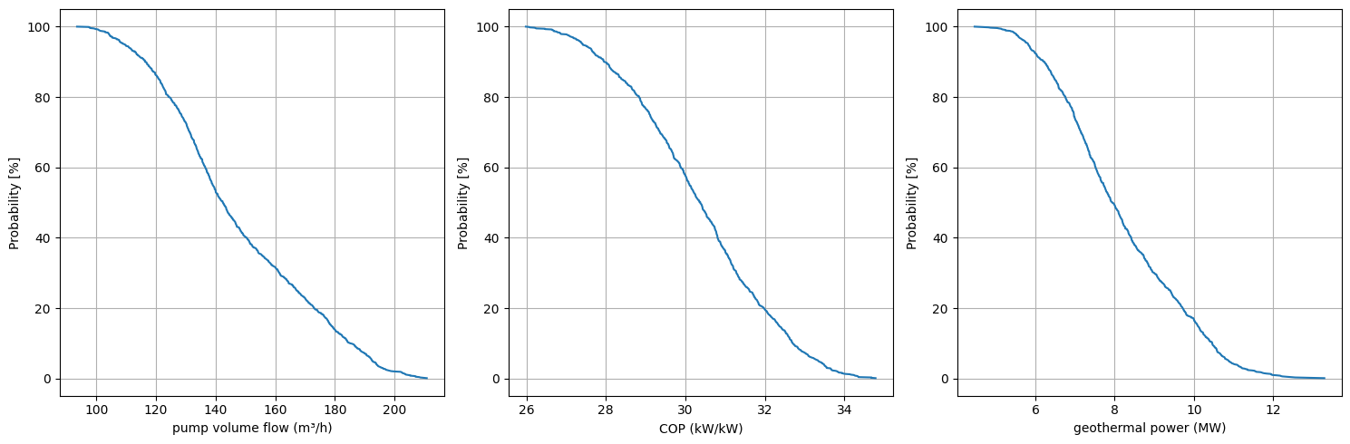
fig, axes = plt.subplots(1,3, figsize=(15,5))

axes[0].plot(data[' pump volume flow (m³/h)'].sort_values(ascending=False).values, np.linspace(0.1,100,len(data)))
axes[1].plot(data[' COP (kW/kW)'].sort_values(ascending=False).values, np.linspace(0.1,100,len(data)))
axes[2].plot(data[' geothermal power (MW)'].sort_values(ascending=False).values, np.linspace(0.1,100,len(data)))

axes[0].grid()
axes[1].grid()
axes[2].grid()

#set label text
axes[0].set_ylabel("Probability [%]")
axes[0].set_xlabel("pump volume flow (m³/h)")

axes[1].set_ylabel("Probability [%]")
axes[1].set_xlabel("COP (kW/kW)")

axes[2].set_ylabel("Probability [%]")
axes[2].set_xlabel("geothermal power (MW)")

plt.tight_layout()