10 Visualizing Spatial Data with PyVista#

Spatial Data can be displayed using the PyVista package. This includes point data, line data and rasters. Data will usually be returned as PolyData datasets or Grids so that the user has the full flexibility of plotting the data with PyVista.

99a42b2a01f94134a4a774765f8051e5

Set File Paths and download Tutorial Data#

If you downloaded the latest GemGIS version from the Github repository, append the path so that the package can be imported successfully. Otherwise, it is recommended to install GemGIS via pip install gemgis and import GemGIS using import gemgis as gg. In addition, the file path to the folder where the data is being stored is set. The tutorial data is downloaded using Pooch (https://www.fatiando.org/pooch/latest/index.html) and stored in the specified folder. Use pip install pooch if Pooch is not installed on your system yet.

[1]:

import gemgis as gg

file_path ='data/10_visualizing_data_with_pyvista/'

[2]:

gg.download_gemgis_data.download_tutorial_data(filename="10_visualizing_data_with_pyvista.zip", dirpath=file_path)

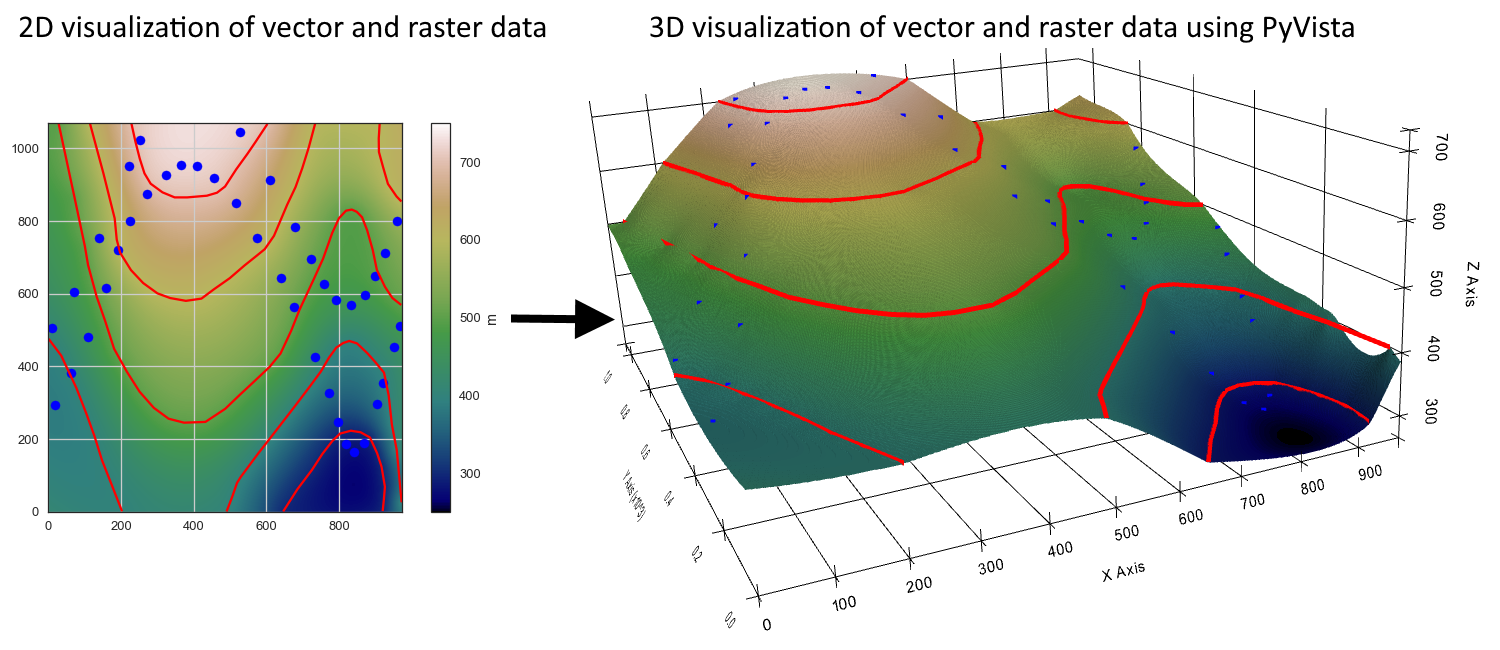
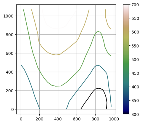
Visualizing Contour Lines with PyVista#

Loading Data#

The contour lines are loaded as Shapely LineStrings within a GeoDataFrame.

[3]:

import pyvista as pv
import geopandas as gpd

contours = gpd.read_file(file_path + 'topo.shp')
contours.head()

[3]:

	id	Z	geometry
0	None	400	LINESTRING (0.74088 475.44101, 35.62873 429.24...
1	None	300	LINESTRING (645.96500 0.52496, 685.14093 61.86...
2	None	400	LINESTRING (490.29223 0.52496, 505.75641 40.73...
3	None	600	LINESTRING (911.43347 1068.58451, 908.85610 10...
4	None	700	LINESTRING (228.43207 1068.58451, 239.77247 10...

Plotting Data#

[4]:

import matplotlib.pyplot as plt

contours.plot(aspect='equal', column='Z', cmap='gist_earth', legend=True)
plt.grid()

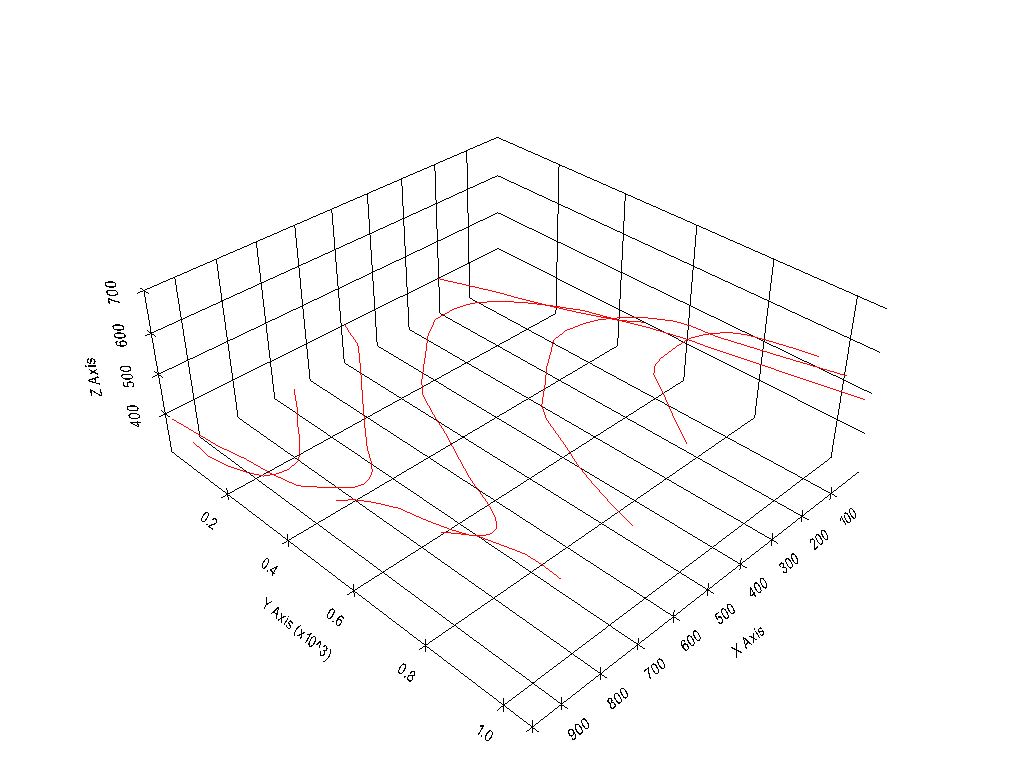
../../_images/getting_started_tutorial_10_visualizing_data_with_pyvista_7_0.png

Extracting the vertices of the contour lines for the plotting with PyVista#

A PolyData dataset of the contour lines can be created using create_lines_3d(..).

[5]:

lines = gg.visualization.create_lines_3d_polydata(gdf=contours)
lines

[5]:

PolyData	Information
N Cells	7
N Points	121
N Strips	0
X Bounds	7.409e-01, 9.717e+02
Y Bounds	5.250e-01, 1.069e+03
Z Bounds	3.000e+02, 7.000e+02
N Arrays	0

[6]:

type(lines)

[6]:

pyvista.core.pointset.PolyData

Plotting the Lines with PyVista#

The result can then be plotted with PyVista by creating a new Plotter and adding the lines as mesh.

[7]:

p = pv.Plotter()

p.add_mesh(mesh=lines, color='red')

p.show_grid(color='black')
p.set_background(color='white')
p.show()

C:\Users\ale93371\Anaconda3\envs\gemgis_test\lib\site-packages\pyvista\jupyter\notebook.py:60: UserWarning: Failed to use notebook backend:

Please install `ipyvtklink` to use this feature: https://github.com/Kitware/ipyvtklink

Falling back to a static output.
  warnings.warn(

../../_images/getting_started_tutorial_10_visualizing_data_with_pyvista_12_1.png

Visualizing Points with PyVista#

Load Data#

The points are loaded as Shapely Points within a GeoDataFrame.

[8]:

import pyvista as pv
import geopandas as gpd
import gemgis as gg

points = gpd.read_file(file_path + 'interfaces_points.shp')
points.head()

[8]:

	id	formation	geometry
0	None	Ton	POINT (19.15013 293.31349)
1	None	Ton	POINT (61.93437 381.45933)
2	None	Ton	POINT (109.35786 480.94557)
3	None	Ton	POINT (157.81230 615.99943)
4	None	Ton	POINT (191.31803 719.09398)

Loading DEM and extract Z values#

In order to plot the points at the correct Z-position, the values have to be extracted from a DEM.

[9]:

import rasterio

dem = rasterio.open(file_path + 'topo.tif')

points_xyz = gg.vector.extract_xyz(gdf=points,
                                   dem=dem)

Plotting Data#

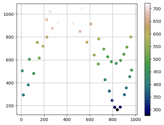
[10]:

import matplotlib.pyplot as plt

points_xyz.plot(aspect='equal', column='Z', cmap='gist_earth', legend=True)
plt.grid()

../../_images/getting_started_tutorial_10_visualizing_data_with_pyvista_18_0.png

Extracting the vertices of the contour lines for the plotting with PyVista#

A PolyData dataset containing the point information can be created using create_points_3d(..).

[11]:

points_mesh = gg.visualization.create_points_3d(gdf=points_xyz)
points_mesh

[11]:

PolyData	Information
N Cells	41
N Points	41
N Strips	0
X Bounds	8.841e+00, 9.661e+02
Y Bounds	1.650e+02, 1.045e+03
Z Bounds	2.769e+02, 7.220e+02
N Arrays	0

[12]:

type(points_mesh)

[12]:

pyvista.core.pointset.PolyData

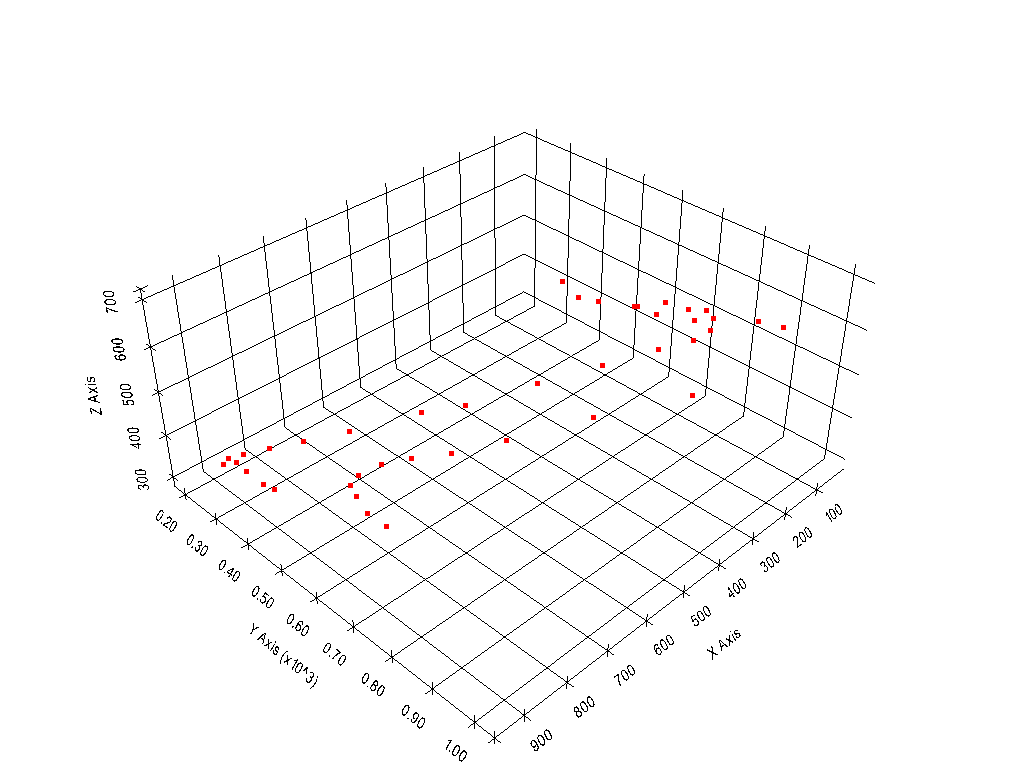
Plotting the Points with PyVista#

The result can then be plotted with PyVista by creating a new Plotter and adding the points as mesh.

[13]:

p = pv.Plotter()

p.add_mesh(mesh=points_mesh, color='red')

p.show_grid(color='black')
p.set_background(color='white')
p.show()

C:\Users\ale93371\Anaconda3\envs\gemgis_test\lib\site-packages\pyvista\jupyter\notebook.py:60: UserWarning: Failed to use notebook backend:

Please install `ipyvtklink` to use this feature: https://github.com/Kitware/ipyvtklink

Falling back to a static output.
  warnings.warn(

../../_images/getting_started_tutorial_10_visualizing_data_with_pyvista_23_1.png

Visualizing the DEM with PyVista#

Loading Data#

The DEM is loaded as Rasterio object using rasterio.

[14]:

import rasterio
import gemgis as gg
import pyvista as pv
import numpy as np

dem = rasterio.open(file_path + 'topo.tif')

dem.read(1)

[14]:

array([[499.90110024, 499.86421238, 499.82858152, ..., 625.37307284,
        625.78164892, 626.18920124],
       [499.53566482, 499.49887905, 499.4633306 , ..., 625.17315916,
        625.58165735, 625.98912699],
       [499.18752484, 499.15158818, 499.11692808, ..., 624.97739453,
        625.38574125, 625.79305697],
       ...,
       [411.5023835 , 411.37335931, 411.24503355, ..., 384.8252337 ,
        386.21293421, 387.56684012],
       [411.66101945, 411.5316941 , 411.40306465, ..., 384.4299191 ,
        385.80964238, 387.15718098],
       [411.82014581, 411.69052091, 411.56158939, ..., 384.04962954,
        385.42140506, 386.76248969]])

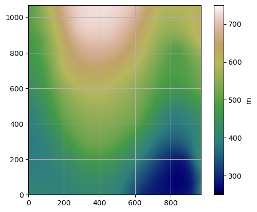
Plotting the Data#

[15]:

import matplotlib.pyplot as plt

im =plt.imshow(dem.read(1), cmap='gist_earth', vmin=250, vmax=750, extent=[0,972,0,1069])
cbar = plt.colorbar(im)
cbar.set_label('m')
plt.grid()

../../_images/getting_started_tutorial_10_visualizing_data_with_pyvista_27_0.png

Converting the Rasterio object or NumPy Array into a Structured Grid#

A StructuredGrid containing the DEM information can be created using create_dem_3d(..).

[16]:

grid = gg.visualization.create_dem_3d(dem=np.flipud(dem.read(1)), extent=[0,972,0,1069])

grid

C:\Users\ale93371\Anaconda3\envs\gemgis_test\lib\site-packages\pyvista\utilities\helpers.py:507: UserWarning: Points is not a float type. This can cause issues when transforming or applying filters. Casting to ``np.float32``. Disable this by passing ``force_float=False``.
  warnings.warn(

[16]:

Header

Data Arrays

StructuredGrid	Information
N Cells	1037028
N Points	1039068
X Bounds	0.000e+00, 9.710e+02
Y Bounds	0.000e+00, 1.068e+03
Z Bounds	2.650e+02, 7.300e+02
Dimensions	1069, 972, 1
N Arrays	1

Name	Field	Type	N Comp	Min	Max
Elevation	Points	float64	1	2.656e+02	7.305e+02

[17]:

type(grid)

[17]:

pyvista.core.pointset.StructuredGrid

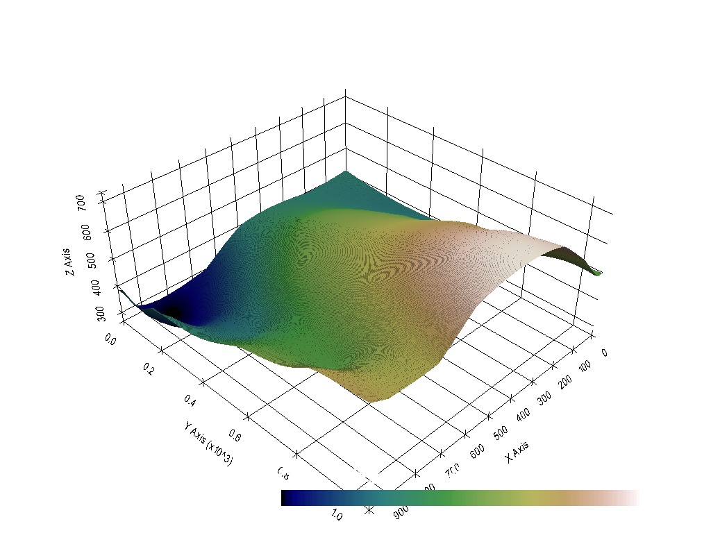
Plotting the Structured Grid with PyVista#

The elevation information of the DEM, also called scalars are stored in the NumPy array grid["Elevation"]. The grid can be plotted by creating a new PyVista Plotter and adding the grid as mesh to the plotter.

[18]:

p = pv.Plotter()

p.add_mesh(mesh=grid, scalars=grid["Elevation"], cmap='gist_earth')

p.show_grid(color='black')
p.set_background(color='white')
p.show()

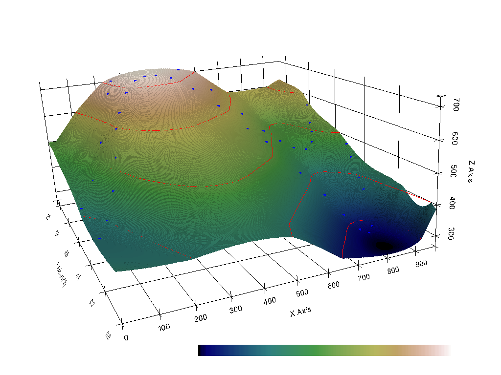
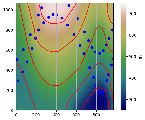
../../_images/getting_started_tutorial_10_visualizing_data_with_pyvista_32_0.png

Combining everything#

All datasets can also be plotted in the same plot.

[19]:

import matplotlib.pyplot as plt

fix, ax = plt.subplots(1,1)
points_xyz.plot(ax=ax, aspect='equal', color='blue')
contours.plot(ax=ax,aspect='equal', color='red')
im =plt.imshow(dem.read(1), cmap='gist_earth', vmin=250, vmax=750, extent=[0,972,0,1069])
cbar = plt.colorbar(im)
cbar.set_label('m')

plt.grid()

../../_images/getting_started_tutorial_10_visualizing_data_with_pyvista_34_0.png

[20]:

p = pv.Plotter()

p.add_mesh(mesh=lines, color='red')

p.add_mesh(mesh=points_mesh, color='blue')

p.add_mesh(mesh=grid, scalars=grid["Elevation"], cmap='gist_earth')

p.camera_position =[(-283.285811675846, -1597.1397046051004, 1155.542325449192),
                    (577.9371599370799, 495.3480261506809, 381.7124055285182),
                    (0.17313457304419916, 0.27814381639313923, 0.9448070898437746)]

p.set_background('white')
p.show_grid(color='black')
p.show()

../../_images/getting_started_tutorial_10_visualizing_data_with_pyvista_35_0.png

GemGIS - Spatial data processing for geomodeling

10 Visualizing Spatial Data with PyVista

Contents

10 Visualizing Spatial Data with PyVista#

Set File Paths and download Tutorial Data#

Visualizing Contour Lines with PyVista#

Loading Data#

Plotting Data#

Extracting the vertices of the contour lines for the plotting with PyVista#

Plotting the Lines with PyVista#

Visualizing Points with PyVista#

Load Data#

Loading DEM and extract Z values#

Plotting Data#

Extracting the vertices of the contour lines for the plotting with PyVista#

Plotting the Points with PyVista#

Visualizing the DEM with PyVista#

Loading Data#

Plotting the Data#

Converting the Rasterio object or NumPy Array into a Structured Grid#

Plotting the Structured Grid with PyVista#

Combining everything#