15 Opening Leapfrog Meshes and GoCAD TSurfaces with GemGIS
Contents
15 Opening Leapfrog Meshes and GoCAD TSurfaces with GemGIS#
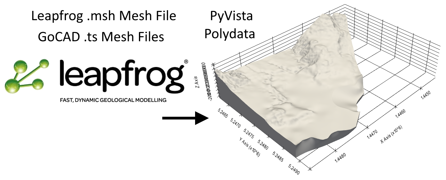
Several different modeling packages store their data in different data types. The following illustrates how to load Leapfrog meshes (.msh-files) and GoCAD TSurfaces (.ts-files) with GemGIS and convert them to a plotable PyVista format.
Set File Paths and download Tutorial Data#
If you downloaded the latest GemGIS version from the Github repository, append the path so that the package can be imported successfully. Otherwise, it is recommended to install GemGIS via pip install gemgis and import GemGIS using import gemgis as gg. In addition, the file path to the folder where the data is being stored is set. The tutorial data is downloaded using Pooch (https://www.fatiando.org/pooch/latest/index.html) and stored in the specified folder. Use
pip install pooch if Pooch is not installed on your system yet.
[1]:
import gemgis as gg

file_path ='data/15_opening_leapfrog_meshes_and_gocad_tsurfaces/'
[2]:
gg.download_gemgis_data.download_tutorial_data(filename="15_opening_leapfrog_meshes_and_gocad_tsurfaces.zip", dirpath=file_path)
Reading Leapfrog Meshes#
Loading the Mesh Data#
The Leapfrog mesh (.msh) is loaded and parsed with read_msh(..). A dictionary containing the face and vertex data will be returned.
[3]:
import numpy as np

data = gg.raster.read_msh(file_path + 'GM_Granodiorite.msh')
[4]:
data
[4]:
{'Tri': array([[    0,     1,     2],
        [    0,     3,     1],
        [    4,     3,     0],
        ...,
        [53677, 53672, 53680],
        [53679, 53677, 53680],
        [53673, 53672, 53677]]),
 'Location': array([[ 1.44625109e+06,  5.24854344e+06, -1.12743862e+02],
        [ 1.44624766e+06,  5.24854640e+06, -1.15102216e+02],
        [ 1.44624808e+06,  5.24854657e+06, -1.15080548e+02],
        ...,
        [ 1.44831008e+06,  5.24896679e+06, -1.24755449e+02],
        [ 1.44830385e+06,  5.24896985e+06, -1.33694397e+02],
        [ 1.44829874e+06,  5.24897215e+06, -1.42506587e+02]])}
[5]:
data.keys()
[5]:
dict_keys(['Tri', 'Location'])
Converting Mesh Data to PyVista PolyData#
The loaded data will now be converted to PyVista PolyData using create_polydata_from_msh(..).
[6]:
surf = gg.visualization.create_polydata_from_msh(data)
surf
[6]:
| Header | Data Arrays | ||||||||||||||||||||||||||||
|---|---|---|---|---|---|---|---|---|---|---|---|---|---|---|---|---|---|---|---|---|---|---|---|---|---|---|---|---|---|
|
|
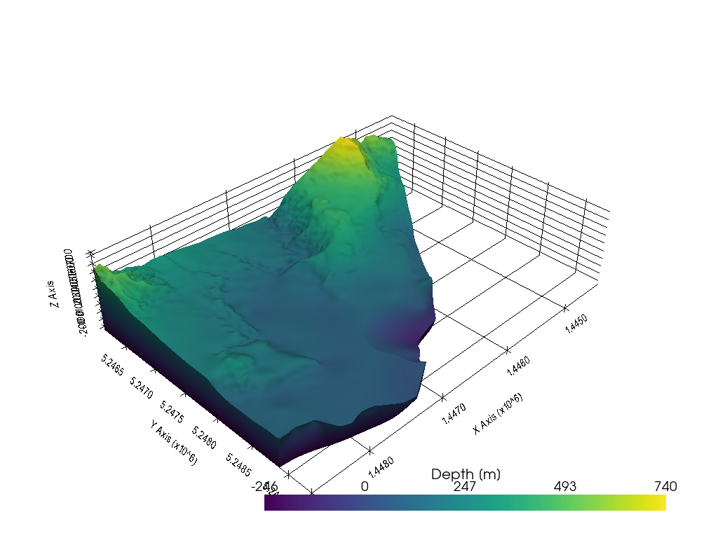
Plotting the data#
Once converted, the data can easily be plotted using PyVista.
[7]:
import pyvista as pv
sargs = dict(fmt="%.0f", color='black')
p = pv.Plotter(notebook=True)

p.add_mesh(surf, scalar_bar_args=sargs)

p.show_grid(color='black')
p.set_background(color='white')
p.show()
C:\Users\ale93371\Anaconda3\envs\gemgis_test\lib\site-packages\pyvista\jupyter\notebook.py:60: UserWarning: Failed to use notebook backend:

Please install `ipyvtklink` to use this feature: https://github.com/Kitware/ipyvtklink

Falling back to a static output.
  warnings.warn(
Reading GoCAD TSurfaces#
Loading the Mesh Data#
The GoCAD mesh (.ts) is loaded and parsed with read_ts(..). An array containing the face data and a DataFrame containing the vertex data will be returned.
Source: KVB Model of the Geological Survey NRW
[8]:
import gemgis as gg
import numpy as np

data = gg.raster.read_ts(file_path + 'KVB_12_Hermann_Katharina.ts')
[9]:
data[0][0]
[9]:
| id | X | Y | Z | aproz | blk | fl | flko | flz1 | flz2 | grs | id_gocad | kenn | vol | vola | |
|---|---|---|---|---|---|---|---|---|---|---|---|---|---|---|---|
| 0 | 0 | 297077.41 | 5677487.26 | -838.50 | 0 | 672132 | 5.01 | 63 | 1777 | 277 | 672 | 6721321830000.00 | 1 | 3156.85 | 3156.85 |
| 1 | 1 | 297437.54 | 5676992.09 | -816.61 | 0 | 672132 | 5.01 | 63 | 1777 | 277 | 672 | 6721321830000.00 | 1 | 3156.85 | 3156.85 |
| 2 | 2 | 298816.17 | 5677906.68 | -590.82 | 0 | 672132 | 5.01 | 63 | 1777 | 277 | 672 | 6721321830000.00 | 1 | 3156.85 | 3156.85 |
| 3 | 3 | 298031.07 | 5678779.55 | -648.69 | 0 | 672132 | 5.01 | 63 | 1777 | 277 | 672 | 6721321830000.00 | 1 | 3156.85 | 3156.85 |
| 4 | 4 | 298852.68 | 5678065.33 | -578.15 | 0 | 672132 | 5.01 | 63 | 1777 | 277 | 672 | 6721321830000.00 | 1 | 3156.85 | 3156.85 |
| 5 | 5 | 298937.09 | 5677681.53 | -586.45 | 0 | 672132 | 5.01 | 63 | 1777 | 277 | 672 | 6721321830000.00 | 1 | 3156.85 | 3156.85 |
| 6 | 6 | 298879.99 | 5677753.93 | -590.39 | 0 | 672132 | 5.01 | 63 | 1777 | 277 | 672 | 6721321830000.00 | 1 | 3156.85 | 3156.85 |
| 7 | 7 | 296511.14 | 5678571.41 | -857.09 | 0 | 672132 | 5.01 | 63 | 1777 | 277 | 672 | 6721321830000.00 | 1 | 3156.85 | 3156.85 |
| 8 | 8 | 296737.27 | 5677981.61 | -857.57 | 0 | 672132 | 5.01 | 63 | 1777 | 277 | 672 | 6721321830000.00 | 1 | 3156.85 | 3156.85 |
| 9 | 9 | 295827.68 | 5680951.57 | -825.33 | 0 | 672132 | 5.01 | 63 | 1777 | 277 | 672 | 6721321830000.00 | 1 | 3156.85 | 3156.85 |
| 10 | 10 | 295622.92 | 5680839.83 | -857.65 | 0 | 672132 | 5.01 | 63 | 1777 | 277 | 672 | 6721321830000.00 | 1 | 3156.85 | 3156.85 |
| 11 | 11 | 298966.25 | 5677660.32 | -583.73 | 0 | 672132 | 5.01 | 63 | 1777 | 277 | 672 | 6721321830000.00 | 1 | 3156.85 | 3156.85 |
| 12 | 12 | 299004.59 | 5677618.71 | -580.85 | 0 | 672132 | 5.01 | 63 | 1777 | 277 | 672 | 6721321830000.00 | 1 | 3156.85 | 3156.85 |
| 13 | 13 | 297014.31 | 5679862.08 | -726.26 | 0 | 672132 | 5.01 | 63 | 1777 | 277 | 672 | 6721321830000.00 | 1 | 3156.85 | 3156.85 |
[10]:
data[1][0]
[10]:
array([[ 0,  1,  2],
       [ 3,  2,  4],
       [ 1,  5,  6],
       [ 3,  7,  8],
       [ 9, 10,  7],
       [ 3,  0,  2],
       [ 1, 11,  5],
       [ 3,  8,  0],
       [ 1, 12, 11],
       [ 3, 13,  7],
       [ 1,  6,  2],
       [13,  9,  7]])
Converting Mesh Data to PyVista PolyData#
The loaded data will now be converted to PyVista PolyData using create_polydata_from_ts(..).
[11]:
surf = gg.visualization.create_polydata_from_ts(data=data, concat=True)
surf.save(file_path + 'mesh.vtk')
surf
[11]:
| Header | Data Arrays | ||||||||||||||||||||||||||||
|---|---|---|---|---|---|---|---|---|---|---|---|---|---|---|---|---|---|---|---|---|---|---|---|---|---|---|---|---|---|
|
|
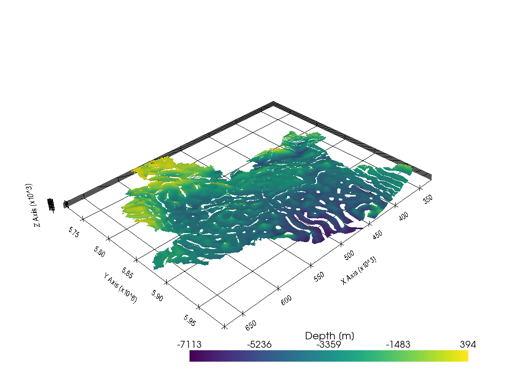
Plotting the data#
Once converted, the data can easily be plotted using PyVista.
[12]:
import pyvista as pv
sargs = dict(fmt="%.0f", color='black')

p = pv.Plotter(notebook=True)

p.add_mesh(surf, scalar_bar_args=sargs)

p.show_grid(color='black')
p.set_background(color='white')
p.show()
C:\Users\ale93371\Anaconda3\envs\gemgis_test\lib\site-packages\pyvista\jupyter\notebook.py:60: UserWarning: Failed to use notebook backend:

Please install `ipyvtklink` to use this feature: https://github.com/Kitware/ipyvtklink

Falling back to a static output.
  warnings.warn(
Extracting Polygons from Faces#
If you would like to display your mesh data or in particular the faces in a GIS, the faces can be converted to Shapely Polygons using create_polygons_from_faces(..). However, each connected surface is now divided in these triangles. The next step is to unify/merge the triangles that belonged to one surface before.
[13]:
polygons = gg.vector.create_polygons_from_faces(mesh=surf, crs='EPSG:25832')
polygons
[13]:
| geometry | |
|---|---|
| 0 | POLYGON Z ((297077.414 5677487.262 -838.496, 2... |
| 1 | POLYGON Z ((298031.070 5678779.547 -648.688, 2... |
| 2 | POLYGON Z ((297437.539 5676992.094 -816.608, 2... |
| 3 | POLYGON Z ((298031.070 5678779.547 -648.688, 2... |
| 4 | POLYGON Z ((295827.680 5680951.574 -825.328, 2... |
| ... | ... |
| 29266 | POLYGON Z ((344329.793 5706418.469 -393.606, 3... |
| 29267 | POLYGON Z ((344329.793 5706418.469 -393.606, 3... |
| 29268 | POLYGON Z ((344329.793 5706418.469 -393.606, 3... |
| 29269 | POLYGON Z ((345667.453 5707314.279 -470.917, 3... |
| 29270 | POLYGON Z ((345667.453 5707314.279 -470.917, 3... |
29271 rows × 1 columns
[14]:
import matplotlib.pyplot as plt

polygons.plot()
plt.grid()

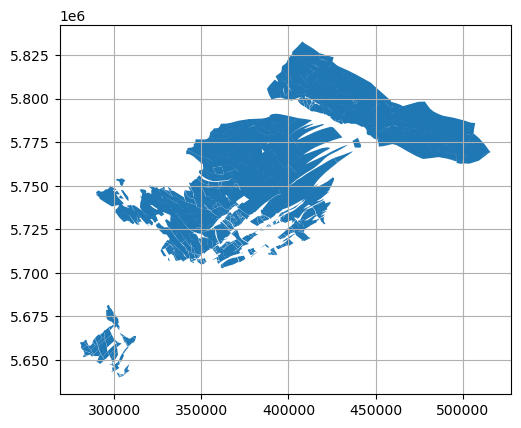
Merging Triangles to Polygons#
Adjacent triangle can now be merged to form single larger polygons using unify_polygons(..).
NB: Currently, Polygons overlapping in their Z dimension are being connected as the underlying Shapely ``unary_union(..)`` function does not account for these overlaps. This was mentioned here: https://github.com/Toblerity/Shapely/issues/1062.
[15]:
polygons = polygons[polygons.is_valid]
polygons_merged = gg.vector.unify_polygons(polygons=polygons)
polygons_merged
[15]:
| geometry | |
|---|---|
| 0 | POLYGON Z ((291580.844 5649724.719 -1109.020, ... |
| 1 | POLYGON Z ((290608.406 5648212.812 -429.361, 2... |
| 2 | POLYGON Z ((290663.789 5649081.398 -611.540, 2... |
| 3 | POLYGON Z ((282206.945 5651577.906 -1157.900, ... |
| 4 | POLYGON Z ((288040.180 5652251.234 -1502.510, ... |
| ... | ... |
| 252 | POLYGON Z ((427861.164 5763280.822 -1735.720, ... |
| 253 | POLYGON Z ((426182.065 5765870.283 -1396.278, ... |
| 254 | POLYGON Z ((429349.305 5785956.133 -1630.430, ... |
| 255 | POLYGON Z ((437544.578 5773703.578 -2109.440, ... |
| 256 | POLYGON Z ((438054.836 5796648.406 -2511.880, ... |
257 rows × 1 columns
[16]:
polygons_merged.plot()
plt.grid()
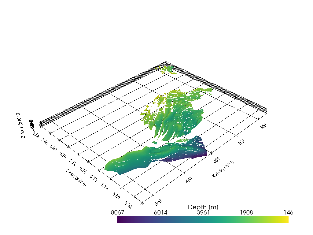
Opening a second dataset with different file structure#
It was encountered that the file structure of TS surfaces of the TUNB model for northern Germany have a different file structure. The code was adapted accordingly and now, both file structures can be opened.
[17]:
data2 = gg.raster.read_ts(file_path + '11_NI_sm.ts')
[18]:
surf2 = gg.visualization.create_polydata_from_ts(data=data2, concat=False)
surf2.save(file_path + 'mesh2.vtk')
surf2
[18]:
| Header | Data Arrays | ||||||||||||||||||||||||||||
|---|---|---|---|---|---|---|---|---|---|---|---|---|---|---|---|---|---|---|---|---|---|---|---|---|---|---|---|---|---|
|
|
[19]:
import pyvista as pv
sargs = dict(fmt="%.0f", color='black')

p = pv.Plotter(notebook=True)

p.add_mesh(surf2, scalar_bar_args=sargs)

p.show_grid(color='black')
p.set_background(color='white')
p.show()
C:\Users\ale93371\Anaconda3\envs\gemgis_test\lib\site-packages\pyvista\jupyter\notebook.py:60: UserWarning: Failed to use notebook backend:

Please install `ipyvtklink` to use this feature: https://github.com/Kitware/ipyvtklink

Falling back to a static output.
  warnings.warn(