35 Plotting Borehole Data with PyVista
Contents
35 Plotting Borehole Data with PyVista#
Borehole data or stratigraphic data can be plotted using GemGIS and PyVista.
Well data provided by the Geological Survey NRW.
Set File Paths and download Tutorial Data#
If you downloaded the latest GemGIS version from the Github repository, append the path so that the package can be imported successfully. Otherwise, it is recommended to install GemGIS via pip install gemgis and import GemGIS using import gemgis as gg. In addition, the file path to the folder where the data is being stored is set. The tutorial data is downloaded using Pooch (https://www.fatiando.org/pooch/latest/index.html) and stored in the specified folder. Use
pip install pooch if Pooch is not installed on your system yet.
[1]:
import gemgis as gg

file_path ='data/35_plotting_borehole_data_with_pyvista/'
WARNING (theano.configdefaults): g++ not available, if using conda: `conda install m2w64-toolchain`
C:\Users\ale93371\Anaconda3\envs\test_gempy\lib\site-packages\theano\configdefaults.py:560: UserWarning: DeprecationWarning: there is no c++ compiler.This is deprecated and with Theano 0.11 a c++ compiler will be mandatory
  warnings.warn("DeprecationWarning: there is no c++ compiler."
WARNING (theano.configdefaults): g++ not detected ! Theano will be unable to execute optimized C-implementations (for both CPU and GPU) and will default to Python implementations. Performance will be severely degraded. To remove this warning, set Theano flags cxx to an empty string.
WARNING (theano.tensor.blas): Using NumPy C-API based implementation for BLAS functions.
[2]:
gg.download_gemgis_data.download_tutorial_data(filename="35_plotting_borehole_data_with_pyvista.zip", dirpath=file_path)
Loading Data#
For better visualization, a mesh is loaded displaying a surface in the subsurface. In addition, sample well data is loaded to demonstrate the visualization of well data.
[2]:
import pyvista as pv
import pandas as pd

mesh = pv.read(file_path + 'base.vtk')
mesh
WARNING (theano.configdefaults): g++ not available, if using conda: `conda install m2w64-toolchain`
C:\Users\ale93371\Anaconda3\envs\test_gempy\lib\site-packages\theano\configdefaults.py:560: UserWarning: DeprecationWarning: there is no c++ compiler.This is deprecated and with Theano 0.11 a c++ compiler will be mandatory
  warnings.warn("DeprecationWarning: there is no c++ compiler."
WARNING (theano.configdefaults): g++ not detected ! Theano will be unable to execute optimized C-implementations (for both CPU and GPU) and will default to Python implementations. Performance will be severely degraded. To remove this warning, set Theano flags cxx to an empty string.
WARNING (theano.tensor.blas): Using NumPy C-API based implementation for BLAS functions.
[2]:
| Header | Data Arrays | ||||||||||||||||||||||||||
|---|---|---|---|---|---|---|---|---|---|---|---|---|---|---|---|---|---|---|---|---|---|---|---|---|---|---|---|
|
|
[3]:
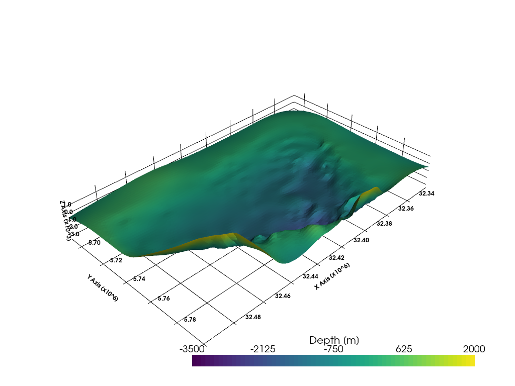
sargs = dict(fmt="%.0f", color='black')

p = pv.Plotter(notebook=True)

p.add_mesh(mesh,scalar_bar_args=sargs, clim=[-3500, 2000])

p.set_background('white')
p.show_grid(color='black')
p.set_scale(1,1,5)
p.show()
[4]:
data = pd.read_csv(file_path + 'Borehole_Data.csv')
data.head()
[4]:
| Unnamed: 0 | Index | Name | X | Y | Z | Altitude | Depth | formation | geometry | |
|---|---|---|---|---|---|---|---|---|---|---|
| 0 | 2091 | GD1017 | ForschungsbohrungMünsterland1 | 32386176.36 | 5763283.15 | 27.00 | 107.00 | 5956.00 | OberCampanium | POINT (32386176.36 5763283.15) |
| 1 | 2092 | GD1017 | ForschungsbohrungMünsterland1 | 32386176.36 | 5763283.15 | -193.00 | 107.00 | 5956.00 | UnterCampanium | POINT (32386176.36 5763283.15) |
| 2 | 2093 | GD1017 | ForschungsbohrungMünsterland1 | 32386176.36 | 5763283.15 | -268.00 | 107.00 | 5956.00 | OberSantonium | POINT (32386176.36 5763283.15) |
| 3 | 2094 | GD1017 | ForschungsbohrungMünsterland1 | 32386176.36 | 5763283.15 | -828.00 | 107.00 | 5956.00 | MittelSantonium | POINT (32386176.36 5763283.15) |
| 4 | 2095 | GD1017 | ForschungsbohrungMünsterland1 | 32386176.36 | 5763283.15 | -988.00 | 107.00 | 5956.00 | UnterSantonium | POINT (32386176.36 5763283.15) |
[5]:
data['formation'].unique()
[5]:
array(['OberCampanium', 'UnterCampanium', 'OberSantonium',
       'MittelSantonium', 'UnterSantonium', 'OberConiacium',
       'UnterConiacium', 'MittelTuronium', 'UnterTuronium',
       'OberCenomanium', 'MittelCenomanium', 'UnterCenomanium',
       'OberAlbium', 'MittelAlbium', 'EssenFM', 'BochumFM', 'WittenFM',
       'Carboniferous', 'Devonian', 'Quaternary', 'MittelConiacium'],
      dtype=object)
Defining Color Dict#
[6]:
color_dict = {
        'OberCampanium':'#3182bd', 'UnterCampanium':'#9ecae1',
        'OberSantonium': '#e6550d', 'MittelSantonium': '#fdae6b', 'UnterSantonium': '#fdd0a2',
        'OberConiacium': '#31a354', 'MittelConiacium': '#74c476', 'UnterConiacium': '#a1d99b',
        'OberTuronium': '#756bb1', 'MittelTuronium': '#9e9ac8', 'UnterTuronium': '#9e9ac8',
        'OberCenomanium': '#636363', 'MittelCenomanium': '#969696', 'UnterCenomanium': '#d9d9d9',
        'OberAlbium': '#637939', 'MittelAlbium': '#8ca252',
        'EssenFM': '#e7969c', 'BochumFM': '#7b4173', 'WittenFM': '#a55194',
        'Carboniferous': '#de9ed6', 'Devonian': '#de9ed6', 'Quaternary': '#de9ed6',
        }
Adding a row to the wells#
[7]:
grouped = data.groupby(['Index'])
df_groups = [grouped.get_group(x) for x in grouped.groups]

list_df = gg.visualization.add_row_to_boreholes(df_groups)

list_df[0].head()
100%|███████████████████████████████████████████████████████████████████████████████████| 2/2 [00:00<00:00, 105.22it/s]
[7]:
| Unnamed: 0 | Index | Name | X | Y | Z | Altitude | Depth | formation | geometry | |
|---|---|---|---|---|---|---|---|---|---|---|
| 0 | nan | GD1017 | ForschungsbohrungMünsterland1 | 32386176.36 | 5763283.15 | 107.00 | 107.00 | 5956.00 | NaN | |
| 0 | 2091.00 | GD1017 | ForschungsbohrungMünsterland1 | 32386176.36 | 5763283.15 | 27.00 | 107.00 | 5956.00 | OberCampanium | POINT (32386176.36 5763283.15) |
| 1 | 2092.00 | GD1017 | ForschungsbohrungMünsterland1 | 32386176.36 | 5763283.15 | -193.00 | 107.00 | 5956.00 | UnterCampanium | POINT (32386176.36 5763283.15) |
| 2 | 2093.00 | GD1017 | ForschungsbohrungMünsterland1 | 32386176.36 | 5763283.15 | -268.00 | 107.00 | 5956.00 | OberSantonium | POINT (32386176.36 5763283.15) |
| 3 | 2094.00 | GD1017 | ForschungsbohrungMünsterland1 | 32386176.36 | 5763283.15 | -828.00 | 107.00 | 5956.00 | MittelSantonium | POINT (32386176.36 5763283.15) |
Creating Lines From Points#
[8]:
lines = gg.visualization.create_lines_from_points(df=list_df[0])
lines
[8]:
| PolyData | Information |
|---|---|
| N Cells | 39 |
| N Points | 20 |
| X Bounds | 3.239e+07, 3.239e+07 |
| Y Bounds | 5.763e+06, 5.763e+06 |
| Z Bounds | -5.849e+03, 1.070e+02 |
| N Arrays | 0 |
Creating Borehole Tubes#
[9]:
tubes, df_groups = gg.visualization.create_borehole_tubes(df=data,
                                               min_length= 10,
                                               radius=1000)
tubes[0]
100%|███████████████████████████████████████████████████████████████████████████████████| 2/2 [00:00<00:00, 153.78it/s]
[9]:
| Header | Data Arrays | ||||||||||||||||||||||||||||||||
|---|---|---|---|---|---|---|---|---|---|---|---|---|---|---|---|---|---|---|---|---|---|---|---|---|---|---|---|---|---|---|---|---|---|
|
|
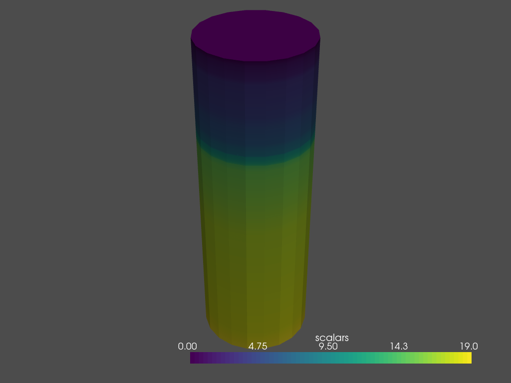
[10]:
tubes[0].plot()
[11]:
labels = gg.visualization.create_borehole_labels(df=data)
labels
[11]:
| Header | Data Arrays | ||||||||||||||||||||||||||
|---|---|---|---|---|---|---|---|---|---|---|---|---|---|---|---|---|---|---|---|---|---|---|---|---|---|---|---|
|
|
Creating Borehole Tube and Labels#
[12]:
tubes, labels, df_groups = gg.visualization.create_boreholes_3d(df=data,
                                                                min_length=10,
                                                                color_dict=color_dict,
                                                                radius=1000)
tubes
100%|███████████████████████████████████████████████████████████████████████████████████| 2/2 [00:00<00:00, 250.10it/s]
[12]:
| Information | Blocks | |||||||||||||||||||
|---|---|---|---|---|---|---|---|---|---|---|---|---|---|---|---|---|---|---|---|---|
|
|
[13]:
tubes[0]
[13]:
| Header | Data Arrays | ||||||||||||||||||||||||||||||||
|---|---|---|---|---|---|---|---|---|---|---|---|---|---|---|---|---|---|---|---|---|---|---|---|---|---|---|---|---|---|---|---|---|---|
|
|
[14]:
labels
[14]:
| Header | Data Arrays | ||||||||||||||||||||||||||
|---|---|---|---|---|---|---|---|---|---|---|---|---|---|---|---|---|---|---|---|---|---|---|---|---|---|---|---|
|
|
[15]:
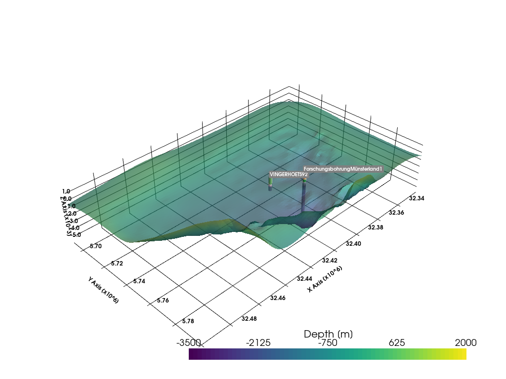
sargs = dict(fmt="%.0f", color='black')

p = pv.Plotter(notebook=True)

p.add_mesh(mesh,scalar_bar_args=sargs, clim=[-3500, 2000], opacity=0.7)
p.add_point_labels(labels, "Labels", point_size=5, font_size=10)
p.add_mesh(tubes, show_scalar_bar=False)

p.set_background('white')
p.show_grid(color='black')
p.set_scale(1,1,5)
p.show()

[16]:
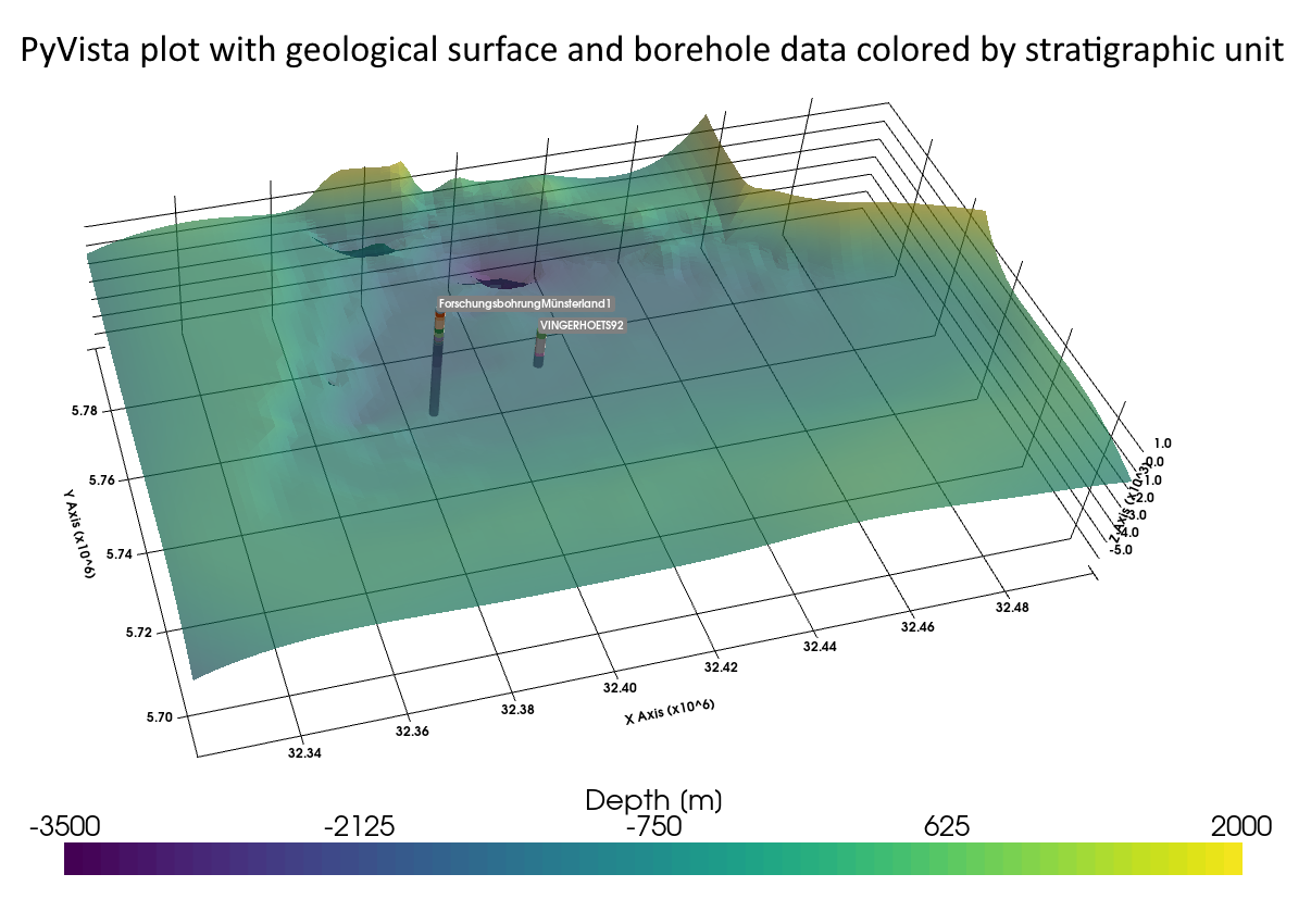
sargs = dict(fmt="%.0f", color='black')

p = pv.Plotter(notebook=True)

p.add_mesh(mesh,scalar_bar_args=sargs, clim=[-3500, 2000], opacity=0.7)
p.add_point_labels(labels, "Labels", point_size=5, font_size=10)

for j in range(len(tubes)):
        df_groups[j] = df_groups[j][1:]
        p.add_mesh(mesh=tubes[j], cmap=[color_dict[i] for i in df_groups[j]['formation'].unique()], show_scalar_bar=False)

p.set_background('white')
p.show_grid(color='black')
p.set_scale(1,1,5)
p.show()