
Example 23 - Planar dipping Layers
Contents
Example 23 - Planar dipping Layers#
This example will show how to convert the geological map below using GemGIS to a GemPy model. This example is based on digitized data. The area is 700 m wide (W-E extent) and 788 m high (N-S extent). The model represents southwards dipping planar layers.
The map has been georeferenced with QGIS. The stratigraphic boundaries were digitized in QGIS. Strikes lines were digitized in QGIS as well and will be used to calculate orientations for the GemPy model. The contour lines were also digitized and will be interpolated with GemGIS to create a topography for the model.
Map Source: Unknown
[1]:
import matplotlib.pyplot as plt
import matplotlib.image as mpimg
img = mpimg.imread('../../getting_started/images/cover_example23.png')
plt.figure(figsize=(10, 10))
imgplot = plt.imshow(img)
plt.axis('off')
plt.tight_layout()
Licensing#
Computational Geosciences and Reservoir Engineering, RWTH Aachen University, Authors: Alexander Juestel. For more information contact: alexander.juestel(at)rwth-aachen.de
This work is licensed under a Creative Commons Attribution 4.0 International License (http://creativecommons.org/licenses/by/4.0/)
Import GemGIS#
If you have installed GemGIS via pip, you can import GemGIS like any other package. If you have downloaded the repository, append the path to the directory where the GemGIS repository is stored and then import GemGIS.
[2]:
import warnings
warnings.filterwarnings("ignore")
import gemgis as gg
Importing Libraries and loading Data#
All remaining packages can be loaded in order to prepare the data and to construct the model. The example data is downloaded form an external server using pooch. It will be stored in a data folder in the same directory where this notebook is stored.
[3]:
import geopandas as gpd
import rasterio
[4]:
file_path = 'data/example23/'
gg.download_gemgis_data.download_tutorial_data(filename="example23_planar_dipping_layers.zip", dirpath=file_path)
Downloading file 'example23_planar_dipping_layers.zip' from 'https://rwth-aachen.sciebo.de/s/AfXRsZywYDbUF34/download?path=%2Fexample23_planar_dipping_layers.zip' to 'C:\Users\ale93371\Documents\gemgis\docs\getting_started\example\data\example23'.
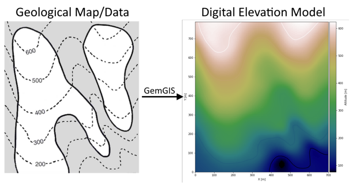
Creating Digital Elevation Model from Contour Lines#
The digital elevation model (DEM) will be created by interpolating contour lines digitized from the georeferenced map using the SciPy Radial Basis Function interpolation wrapped in GemGIS. The respective function used for that is gg.vector.interpolate_raster().
[5]:
img = mpimg.imread('../../getting_started/images/dem_example23.png')
plt.figure(figsize=(10, 10))
imgplot = plt.imshow(img)
plt.axis('off')
plt.tight_layout()
[6]:
topo = gpd.read_file(file_path + 'topo23.shp')
topo.head()
[6]:
| id | Z | geometry | |
|---|---|---|---|
| 0 | None | 600 | LINESTRING (15.116 787.112, 22.878 758.803, 29... |
| 1 | None | 600 | LINESTRING (450.485 786.656, 457.791 773.642, ... |
| 2 | None | 500 | LINESTRING (1.189 660.177, 11.235 642.598, 21.... |
| 3 | None | 400 | LINESTRING (0.790 532.842, 12.776 506.360, 26.... |
| 4 | None | 300 | LINESTRING (3.872 351.115, 20.310 331.025, 34.... |
Interpolating the contour lines#
[7]:
topo_raster = gg.vector.interpolate_raster(gdf=topo, value='Z', method='rbf', res=5)
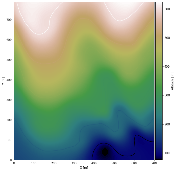
Plotting the raster#
[8]:
import matplotlib.pyplot as plt

from mpl_toolkits.axes_grid1 import make_axes_locatable

fix, ax = plt.subplots(1, figsize=(10,10))
topo.plot(ax=ax, aspect='equal', column='Z', cmap='gist_earth')
im = ax.imshow(topo_raster, origin='lower', extent=[0,700,0,788], cmap='gist_earth')
divider = make_axes_locatable(ax)
cax = divider.append_axes("right", size="5%", pad=0.05)
cbar = plt.colorbar(im, cax=cax)
cbar.set_label('Altitude [m]')
ax.set_xlabel('X [m]')
ax.set_ylabel('Y [m]')
[8]:
Text(98.40090121128625, 0.5, 'Y [m]')
Saving the raster to disc#
After the interpolation of the contour lines, the raster is saved to disc using gg.raster.save_as_tiff(). The function will not be executed as as raster is already provided with the example data.
Opening Raster#
The previously computed and saved raster can now be opened using rasterio.
[9]:
topo_raster = rasterio.open(file_path + 'raster23.tif')
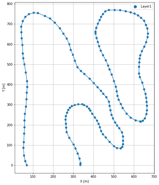
Interface Points of stratigraphic boundaries#
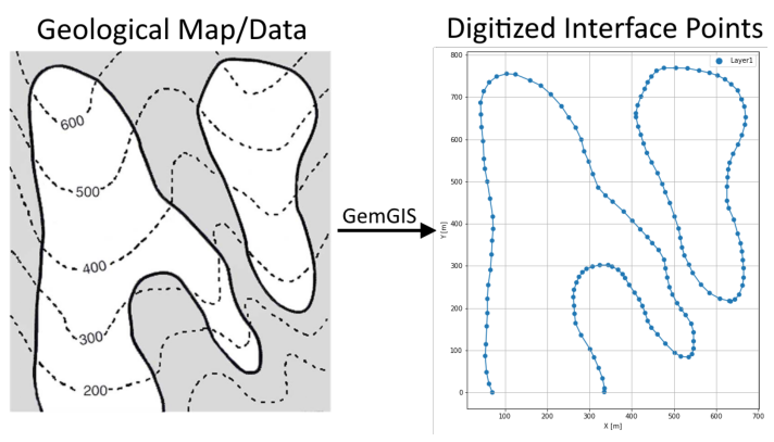
The interface points will be extracted from LineStrings digitized from the georeferenced map using QGIS. It is important to provide a formation name for each layer boundary. The vertical position of the interface point will be extracted from the digital elevation model using the GemGIS function gg.vector.extract_xyz(). The resulting GeoDataFrame now contains single points including the information about the respective formation.
[10]:
img = mpimg.imread('../../getting_started/images/interfaces_example23.png')
plt.figure(figsize=(10, 10))
imgplot = plt.imshow(img)
plt.axis('off')
plt.tight_layout()
[11]:
interfaces = gpd.read_file(file_path + 'interfaces23.shp')
interfaces.head()
[11]:
| id | formation | geometry | |
|---|---|---|---|
| 0 | None | Layer1 | LINESTRING (70.166 0.062, 62.317 20.308, 56.38... |
| 1 | None | Layer1 | LINESTRING (631.470 216.874, 609.097 222.125, ... |
Extracting XY coordinates from Digital Elevation Model#
[12]:
interfaces_coords = gg.vector.extract_xyz(gdf=interfaces, dem=topo_raster)
interfaces_coords = interfaces_coords.sort_values(by='formation', ascending=False)
interfaces_coords.head()
[12]:
| formation | geometry | X | Y | Z | |
|---|---|---|---|---|---|
| 0 | Layer1 | POINT (70.166 0.062) | 70.17 | 0.06 | 166.32 |
| 107 | Layer1 | POINT (472.573 494.031) | 472.57 | 494.03 | 393.99 |
| 100 | Layer1 | POINT (524.854 324.632) | 524.85 | 324.63 | 289.36 |
| 101 | Layer1 | POINT (519.147 343.581) | 519.15 | 343.58 | 294.85 |
| 102 | Layer1 | POINT (515.265 366.411) | 515.27 | 366.41 | 304.13 |
Plotting the Interface Points#
[13]:
fig, ax = plt.subplots(1, figsize=(10,10))

interfaces.plot(ax=ax, column='formation', legend=True, aspect='equal')
interfaces_coords.plot(ax=ax, column='formation', legend=True, aspect='equal')
plt.grid()
plt.xlabel('X [m]')
plt.ylabel('Y [m]')
[13]:
Text(116.99284374939245, 0.5, 'Y [m]')
Orientations from Strike Lines#
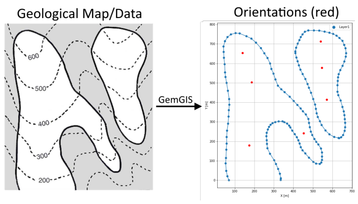
Strike lines connect outcropping stratigraphic boundaries (interfaces) of the same altitude. In other words: the intersections between topographic contours and stratigraphic boundaries at the surface. The height difference and the horizontal difference between two digitized lines is used to calculate the dip and azimuth and hence an orientation that is necessary for GemPy. In order to calculate the orientations, each set of strikes lines/LineStrings for one formation must be given an id
number next to the altitude of the strike line. The id field is already predefined in QGIS. The strike line with the lowest altitude gets the id number 1, the strike line with the highest altitude the the number according to the number of digitized strike lines. It is currently recommended to use one set of strike lines for each structural element of one formation as illustrated.
[14]:
img = mpimg.imread('../../getting_started/images/orientations_example23.png')
plt.figure(figsize=(10, 10))
imgplot = plt.imshow(img)
plt.axis('off')
plt.tight_layout()
[15]:
strikes = gpd.read_file(file_path + 'strikes23.shp')
strikes
[15]:
| id | Z | formation | geometry | |
|---|---|---|---|---|
| 0 | 3 | 600 | Layer1a | LINESTRING (46.044 702.206, 190.042 725.406) |
| 1 | 2 | 500 | Layer1a | LINESTRING (49.510 572.074, 271.908 618.474) |
| 2 | 1 | 400 | Layer1a | LINESTRING (69.244 368.876, 355.641 452.075) |
| 3 | 2 | 300 | Layer1b | LINESTRING (62.310 272.344, 266.042 247.811) |
| 4 | 1 | 200 | Layer1b | LINESTRING (54.844 118.745, 312.974 79.279) |
| 5 | 2 | 300 | Layer1c | LINESTRING (391.907 261.677, 459.106 340.610) |
| 6 | 1 | 200 | Layer1c | LINESTRING (436.706 178.478, 524.172 187.011) |
| 7 | 4 | 600 | Layer1d | LINESTRING (463.373 765.139, 612.705 747.006) |
| 8 | 3 | 500 | Layer1d | LINESTRING (412.173 672.340, 670.304 668.073) |
| 9 | 2 | 400 | Layer1d | LINESTRING (471.906 495.275, 625.505 476.075) |
| 10 | 1 | 300 | Layer1d | LINESTRING (519.906 352.343, 662.838 332.077) |
Calculate Orientations for each formation#
[16]:
orientations_layer1a = gg.vector.calculate_orientations_from_strike_lines(gdf=strikes[strikes['formation']=='Layer1a'].sort_values(by='Z', ascending=True).reset_index())
orientations_layer1a
[16]:
| dip | azimuth | Z | geometry | polarity | formation | X | Y | |
|---|---|---|---|---|---|---|---|---|
| 0 | 28.63 | 165.42 | 450.00 | POINT (186.576 502.875) | 1.00 | Layer1a | 186.58 | 502.87 |
| 1 | 39.48 | 168.98 | 550.00 | POINT (139.376 654.540) | 1.00 | Layer1a | 139.38 | 654.54 |
[17]:
orientations_layer1b = gg.vector.calculate_orientations_from_strike_lines(gdf=strikes[strikes['formation']=='Layer1b'].sort_values(by='Z', ascending=True).reset_index())
orientations_layer1b
[17]:
| dip | azimuth | Z | geometry | polarity | formation | X | Y | |
|---|---|---|---|---|---|---|---|---|
| 0 | 33.10 | 187.99 | 250.00 | POINT (174.042 179.545) | 1.00 | Layer1b | 174.04 | 179.54 |
[18]:
orientations_layer1c = gg.vector.calculate_orientations_from_strike_lines(gdf=strikes[strikes['formation']=='Layer1c'].sort_values(by='Z', ascending=True).reset_index())
orientations_layer1c
[18]:
| dip | azimuth | Z | geometry | polarity | formation | X | Y | |
|---|---|---|---|---|---|---|---|---|
| 0 | 46.62 | 148.69 | 250.00 | POINT (452.973 241.944) | 1.00 | Layer1c | 452.97 | 241.94 |
[19]:
orientations_layer1d = gg.vector.calculate_orientations_from_strike_lines(gdf=strikes[strikes['formation']=='Layer1d'].sort_values(by='Z', ascending=True).reset_index())
orientations_layer1d
[19]:
| dip | azimuth | Z | geometry | polarity | formation | X | Y | |
|---|---|---|---|---|---|---|---|---|
| 0 | 36.35 | 187.56 | 350.00 | POINT (570.038 413.942) | 1.00 | Layer1d | 570.04 | 413.94 |
| 1 | 29.60 | 182.57 | 450.00 | POINT (544.972 577.941) | 1.00 | Layer1d | 544.97 | 577.94 |
| 2 | 52.06 | 182.45 | 550.00 | POINT (539.639 713.139) | 1.00 | Layer1d | 539.64 | 713.14 |
Merging Orientations#
[20]:
import pandas as pd
orientations = pd.concat([orientations_layer1a, orientations_layer1b, orientations_layer1c, orientations_layer1d]).reset_index()
orientations['formation'] = 'Layer1'
orientations
[20]:
| index | dip | azimuth | Z | geometry | polarity | formation | X | Y | |
|---|---|---|---|---|---|---|---|---|---|
| 0 | 0 | 28.63 | 165.42 | 450.00 | POINT (186.576 502.875) | 1.00 | Layer1 | 186.58 | 502.87 |
| 1 | 1 | 39.48 | 168.98 | 550.00 | POINT (139.376 654.540) | 1.00 | Layer1 | 139.38 | 654.54 |
| 2 | 0 | 33.10 | 187.99 | 250.00 | POINT (174.042 179.545) | 1.00 | Layer1 | 174.04 | 179.54 |
| 3 | 0 | 46.62 | 148.69 | 250.00 | POINT (452.973 241.944) | 1.00 | Layer1 | 452.97 | 241.94 |
| 4 | 0 | 36.35 | 187.56 | 350.00 | POINT (570.038 413.942) | 1.00 | Layer1 | 570.04 | 413.94 |
| 5 | 1 | 29.60 | 182.57 | 450.00 | POINT (544.972 577.941) | 1.00 | Layer1 | 544.97 | 577.94 |
| 6 | 2 | 52.06 | 182.45 | 550.00 | POINT (539.639 713.139) | 1.00 | Layer1 | 539.64 | 713.14 |
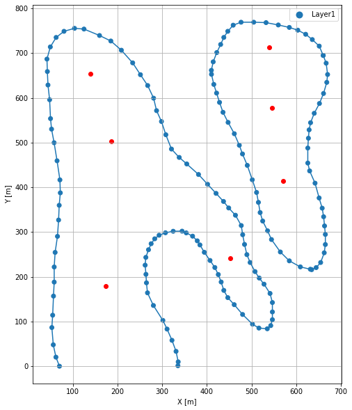
Plotting the Orientations#
[21]:
fig, ax = plt.subplots(1, figsize=(10,10))

interfaces.plot(ax=ax, column='formation', legend=True, aspect='equal')
interfaces_coords.plot(ax=ax, column='formation', legend=True, aspect='equal')
orientations.plot(ax=ax, color='red', aspect='equal')
plt.grid()
plt.xlabel('X [m]')
plt.ylabel('Y [m]')
[21]:
Text(116.99284374939245, 0.5, 'Y [m]')
GemPy Model Construction#
The structural geological model will be constructed using the GemPy package.
[22]:
import gempy as gp
WARNING (theano.configdefaults): g++ not available, if using conda: `conda install m2w64-toolchain`
WARNING (theano.configdefaults): g++ not detected ! Theano will be unable to execute optimized C-implementations (for both CPU and GPU) and will default to Python implementations. Performance will be severely degraded. To remove this warning, set Theano flags cxx to an empty string.
WARNING (theano.tensor.blas): Using NumPy C-API based implementation for BLAS functions.
Creating new Model#
[23]:
geo_model = gp.create_model('Model23')
geo_model
[23]:
Model23 2022-04-07 09:15
Initiate Data#
[24]:
gp.init_data(geo_model, [0,700,0,788,0,400], [100,100,100],
             surface_points_df = interfaces_coords[interfaces_coords['Z']!=0].sample(n=100),
             orientations_df = orientations,
             default_values=True)
Active grids: ['regular']
[24]:
Model23 2022-04-07 09:15
Model Surfaces#
[25]:
geo_model.surfaces
[25]:
| surface | series | order_surfaces | color | id | |
|---|---|---|---|---|---|
| 0 | Layer1 | Default series | 1 | #015482 | 1 |
Mapping the Stack to Surfaces#
[26]:
gp.map_stack_to_surfaces(geo_model,
                         {
                          'Strata1': ('Layer1'),
                         },
                         remove_unused_series=True)
geo_model.add_surfaces('Basement')
[26]:
| surface | series | order_surfaces | color | id | |
|---|---|---|---|---|---|
| 0 | Layer1 | Strata1 | 1 | #015482 | 1 |
| 1 | Basement | Strata1 | 2 | #9f0052 | 2 |
Showing the Number of Data Points#
[27]:
gg.utils.show_number_of_data_points(geo_model=geo_model)
[27]:
| surface | series | order_surfaces | color | id | No. of Interfaces | No. of Orientations | |
|---|---|---|---|---|---|---|---|
| 0 | Layer1 | Strata1 | 1 | #015482 | 1 | 100 | 7 |
| 1 | Basement | Strata1 | 2 | #9f0052 | 2 | 0 | 0 |
Loading Digital Elevation Model#
[28]:
geo_model.set_topography(
    source='gdal', filepath=file_path + 'raster23.tif')
Cropped raster to geo_model.grid.extent.
depending on the size of the raster, this can take a while...
storing converted file...
Active grids: ['regular' 'topography']
[28]:
Grid Object. Values:
array([[  3.5       ,   3.94      ,   2.        ],
       [  3.5       ,   3.94      ,   6.        ],
       [  3.5       ,   3.94      ,  10.        ],
       ...,
       [697.5       , 775.53164557, 559.49066162],
       [697.5       , 780.51898734, 563.62854004],
       [697.5       , 785.50632911, 567.61871338]])
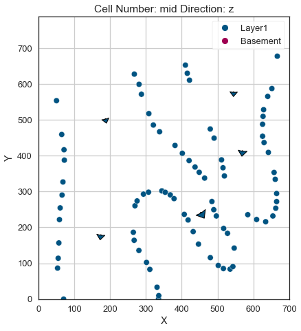
Plotting Input Data#
[29]:
gp.plot_2d(geo_model, direction='z', show_lith=False, show_boundaries=False)
plt.grid()
[30]:
gp.plot_3d(geo_model, image=False, plotter_type='basic', notebook=True)
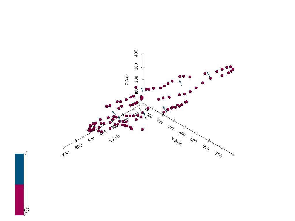
[30]:
<gempy.plot.vista.GemPyToVista at 0x167bcc5b100>
Setting the Interpolator#
[31]:
gp.set_interpolator(geo_model,
                    compile_theano=True,
                    theano_optimizer='fast_compile',
                    verbose=[],
                    update_kriging = False
                    )
Compiling theano function...
Level of Optimization:  fast_compile
Device:  cpu
Precision:  float64
Number of faults:  0
Compilation Done!
Kriging values:
                   values
range            1127.36
$C_o$           30260.57
drift equations      [3]
[31]:
<gempy.core.interpolator.InterpolatorModel at 0x167b4d80430>
Computing Model#
[32]:
sol = gp.compute_model(geo_model, compute_mesh=True)
Plotting Cross Sections#
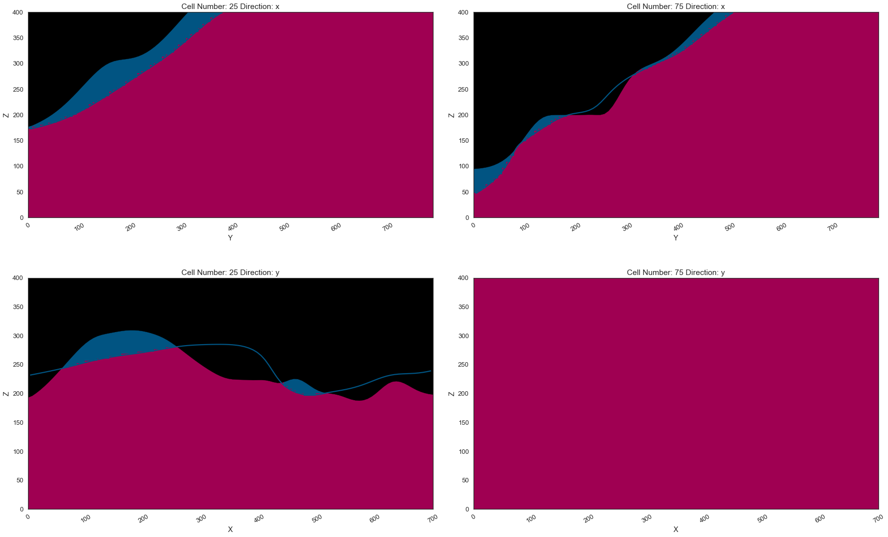
[33]:
gp.plot_2d(geo_model, direction=['x', 'x', 'y', 'y'], cell_number=[25,75,25,75], show_topography=True, show_data=False)
[33]:
<gempy.plot.visualization_2d.Plot2D at 0x167bc470160>
Plotting 3D Model#
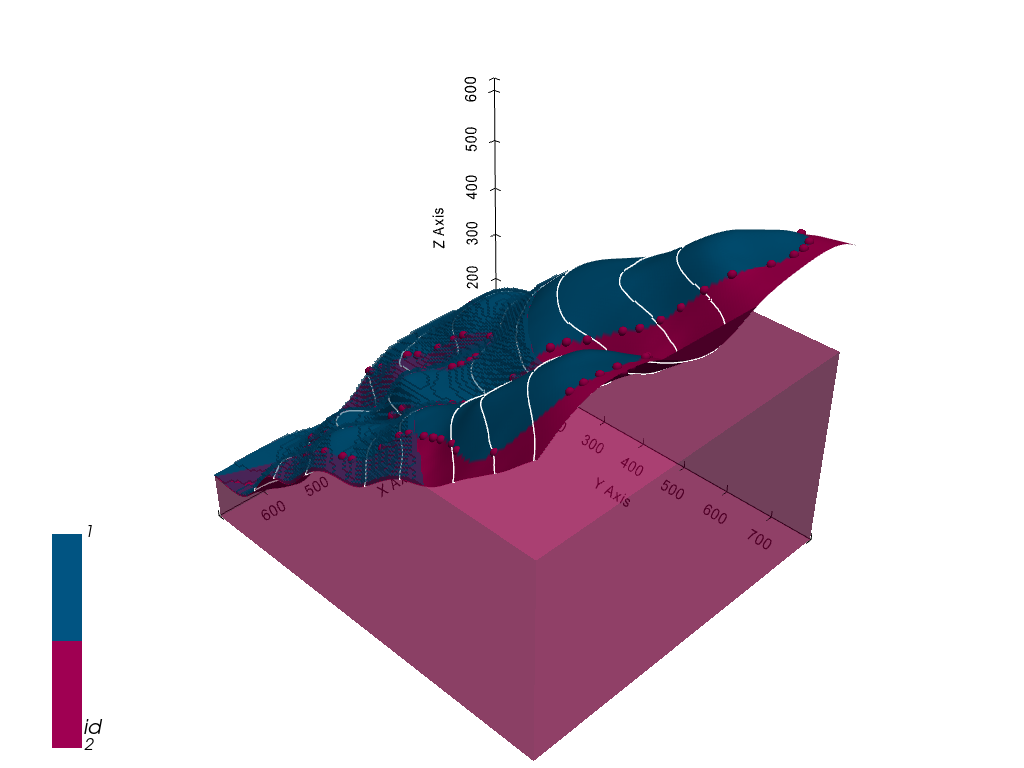
[34]:
gpv = gp.plot_3d(geo_model, image=False, show_topography=True,
                 plotter_type='basic', notebook=True, show_lith=True)
[ ]: