14 Visualizing Topography and Maps with PyVista
Contents
14 Visualizing Topography and Maps with PyVista#
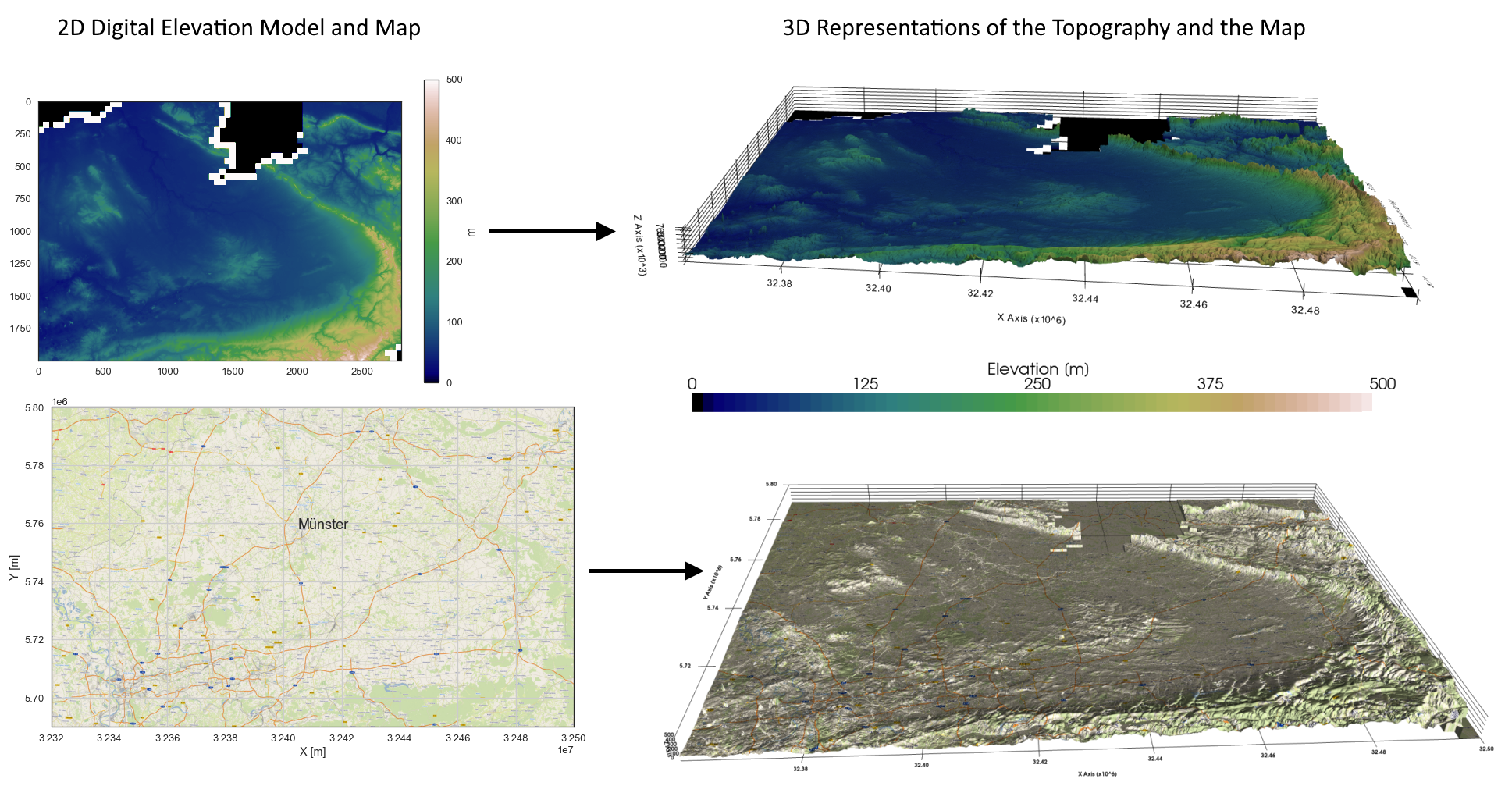
The topography of an area can be visualized in 3D with PyVista and additional maps can also be draped over the topography.
Set File Paths and download Tutorial Data#
If you downloaded the latest GemGIS version from the Github repository, append the path so that the package can be imported successfully. Otherwise, it is recommended to install GemGIS via pip install gemgis and import GemGIS using import gemgis as gg. In addition, the file path to the folder where the data is being stored is set. The tutorial data is downloaded using Pooch (https://www.fatiando.org/pooch/latest/index.html) and stored in the specified folder. Use
pip install pooch if Pooch is not installed on your system yet.
[1]:
import gemgis as gg

file_path ='data/14_visualizing_topography_and_maps_with_pyvista/'
[2]:
gg.download_gemgis_data.download_tutorial_data(filename="14_visualizing_topography_and_maps_with_pyvista.zip", dirpath=file_path)
Downloading file '14_visualizing_topography_and_maps_with_pyvista.zip' from 'https://rwth-aachen.sciebo.de/s/AfXRsZywYDbUF34/download?path=%2F14_visualizing_topography_and_maps_with_pyvista.zip' to 'C:\Users\ale93371\Documents\gemgis\docs\getting_started\tutorial\data\14_visualizing_topography_and_maps_with_pyvista'.
Loading the data#
A 50 m DEM of the Münsterland Basin is loaded to illustrate the visualizing of topography in PyVista. The data will be used under Datenlizenz Deutschland – Zero – Version 2.0. It was obtained from the WCS Service https://www.wcs.nrw.de/geobasis/wcs_nw_dgm. The data will automatically be converted to a StructuredGrid with Elevation [m] as data array.
[3]:
import pyvista as pv

mesh = gg.visualization.read_raster(path=file_path + 'DEM50.tif',
                                    nodata_val=9999.0,
                                    name='Elevation [m]')

mesh
[3]:
| Header | Data Arrays | ||||||||||||||||||||||||||||
|---|---|---|---|---|---|---|---|---|---|---|---|---|---|---|---|---|---|---|---|---|---|---|---|---|---|---|---|---|---|
|
|
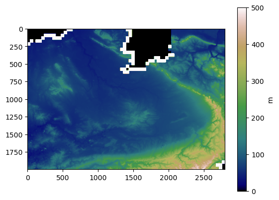
Plotting the data in 2D#
[4]:
import rasterio

dem = rasterio.open(file_path + 'DEM50.tif')
dem.read(1)
[4]:
array([[  0.  ,   0.  ,   0.  , ...,  40.1 ,  40.09,  44.58],
       [  0.  ,   0.  ,   0.  , ...,  40.08,  40.07,  44.21],
       [  0.  ,   0.  ,   0.  , ...,  40.14,  44.21,  43.98],
       ...,
       [100.56, 102.14, 102.17, ...,   0.  ,   0.  ,   0.  ],
       [ 99.44,  99.85,  99.77, ...,   0.  ,   0.  ,   0.  ],
       [ 88.32,  91.76,  98.68, ...,   0.  ,   0.  ,   0.  ]],
      dtype=float32)
[5]:
import matplotlib.pyplot as plt

im = plt.imshow(dem.read(1), cmap='gist_earth', vmin=0, vmax=500)
cbar = plt.colorbar(im)
cbar.set_label('m')
Wrap Mesh by Scalars#
The dataset’s points are wrapped by a point data scalars array’s values.
[6]:
topo = mesh.warp_by_scalar(scalars="Elevation [m]", factor=15.0)

topo
[6]:
| Header | Data Arrays | ||||||||||||||||||||||||||||
|---|---|---|---|---|---|---|---|---|---|---|---|---|---|---|---|---|---|---|---|---|---|---|---|---|---|---|---|---|---|
|
|
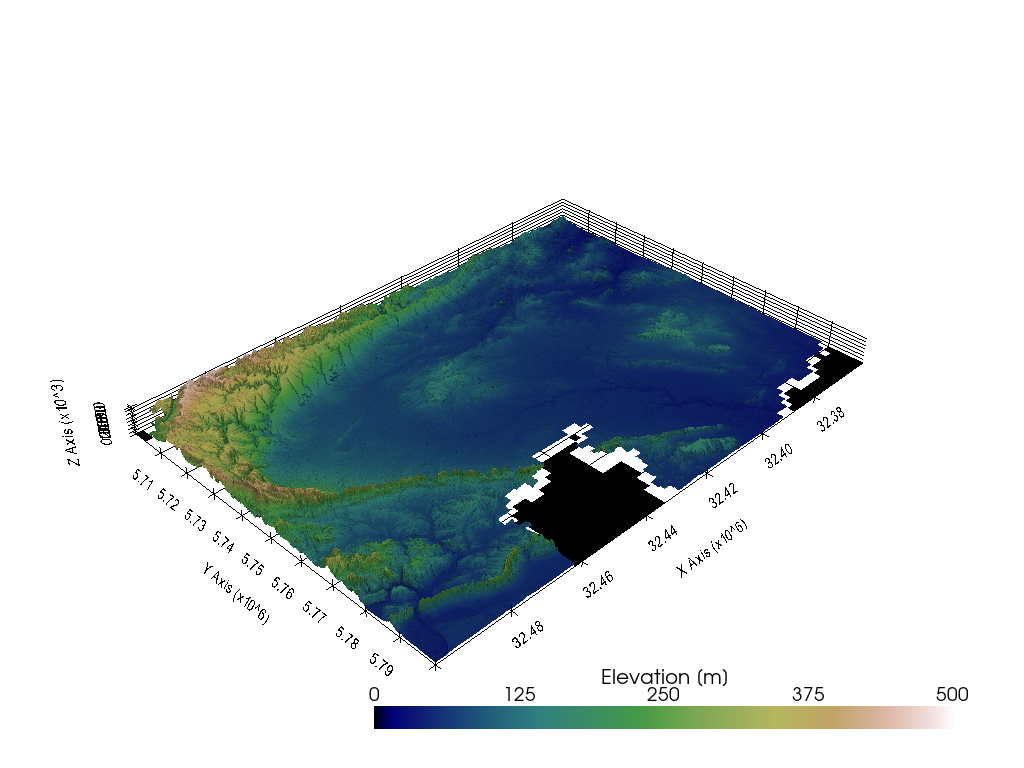
Plotting the Mesh#
The mesh can then easily be plotted with PyVista
[7]:
sargs = dict(fmt="%.0f", color='black')


p = pv.Plotter(notebook=True)
p.add_mesh(mesh=topo, cmap='gist_earth', scalar_bar_args=sargs, clim=[-0, 500])

p.set_background('white')
p.show_grid(color='black')
p.show()
C:\Users\ale93371\Anaconda3\envs\gemgis_test\lib\site-packages\pyvista\jupyter\notebook.py:60: UserWarning: Failed to use notebook backend:

Please install `ipyvtklink` to use this feature: https://github.com/Kitware/ipyvtklink

Falling back to a static output.
  warnings.warn(
Drape Topographic map over Digital Elevation Model#
It is also possible to drape a topographic map over the digital elevation model. The map will be loaded from a WMS service which will be introduced in a later tutorial in more detail. In order to make the feature work, the width and the height of both, the map data and the digital elevation model, must be the same!
Loading the WMS Service#
[8]:
wms_map = gg.web.load_as_array('https://ows.terrestris.de/osm/service?',
                             'OSM-WMS', 'default', 'EPSG:4647', [32320000,32500000, 5690000, 5800000], [2800, 2000], 'image/png')
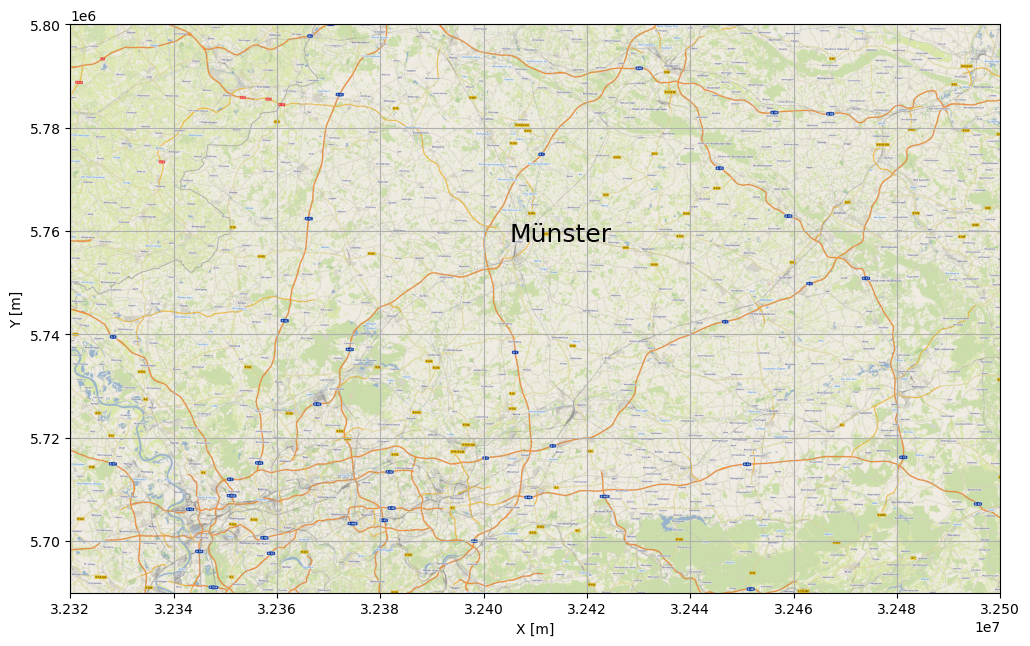
Plotting the map data#
[9]:
import matplotlib.pyplot as plt

plt.figure(figsize = (12,12))
plt.imshow(wms_map, extent= [32320000,32500000, 5690000, 5800000])
plt.grid()
plt.ylabel('Y [m]')
plt.xlabel('X [m]')
plt.text(32405000,5758000, 'Münster', size = 18)
[9]:
Text(32405000, 5758000, 'Münster')
Converting the array values to RGB values#
When downloading the wms_map, a total of three bands are downloaded. These array values need to be converted to RGB values.
[10]:
wms_map[0]
[10]:
array([[0.35686275, 0.35686275, 0.48235294, 1.        ],
       [0.40392157, 0.40784314, 0.52156866, 1.        ],
       [0.92941177, 0.92941177, 0.94509804, 1.        ],
       ...,
       [0.59607846, 0.69803923, 0.8       , 1.        ],
       [0.6156863 , 0.69411767, 0.76862746, 1.        ],
       [0.8784314 , 0.8666667 , 0.8156863 , 1.        ]], dtype=float32)
[11]:
wms_map.shape
[11]:
(2000, 2800, 4)
[12]:
wms_stacked = gg.visualization.convert_to_rgb(array=wms_map)

wms_stacked[:2]
[12]:
array([[[ 91,  91, 123],
        [103, 104, 133],
        [237, 237, 241],
        ...,
        [152, 178, 204],
        [157, 177, 196],
        [224, 221, 208]],

       [[255, 255, 255],
        [255, 255, 255],
        [247, 248, 243],
        ...,
        [150, 178, 206],
        [171, 175, 170],
        [250, 249, 243]]], dtype=uint8)
[13]:
wms_stacked.shape
[13]:
(2000, 2800, 3)
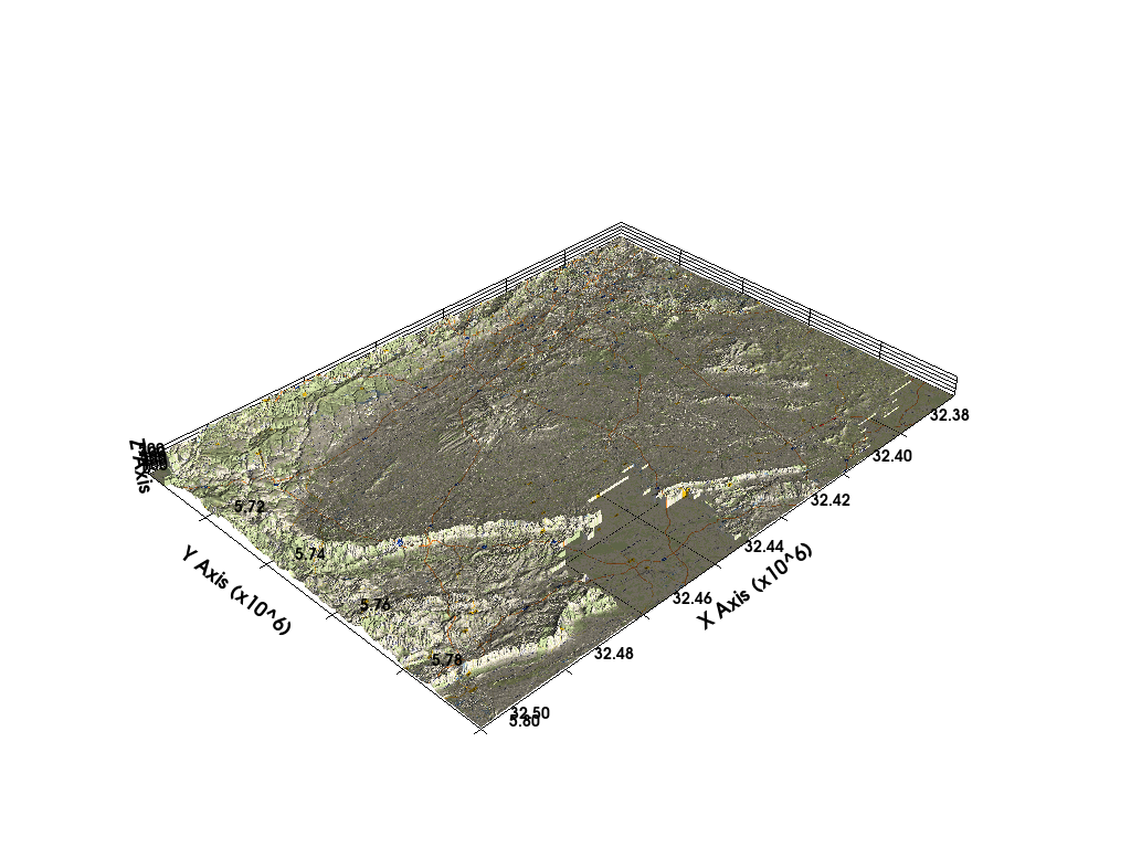
Draping the array over the Digital Elevation Model#
The map data of the WMS map can be draped over the digital elevation model.
[14]:
mesh, texture = gg.visualization.drape_array_over_dem(array=wms_stacked,
                                                      dem=dem)
[15]:
mesh
[15]:
| Header | Data Arrays | ||||||||||||||||||||||||||||
|---|---|---|---|---|---|---|---|---|---|---|---|---|---|---|---|---|---|---|---|---|---|---|---|---|---|---|---|---|---|
|
|
[16]:
texture
[16]:
<Texture(0x00000232440EFCF0) at 0x000002320E0786A0>
Plotting the data in PyVista#
[17]:
sargs = dict(fmt="%.0f", color='black')


p = pv.Plotter(notebook=True)
p.add_mesh(mesh=mesh, cmap='gist_earth', scalar_bar_args=sargs, texture=texture)

p.set_background('white')
p.show_grid(color='black')
p.set_scale(1,1,10)
p.show()