
Example 24- Unconformable Layers
Contents
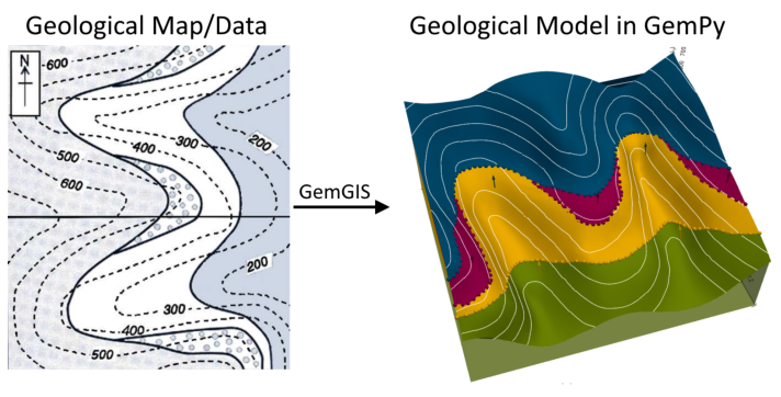
Example 24- Unconformable Layers#
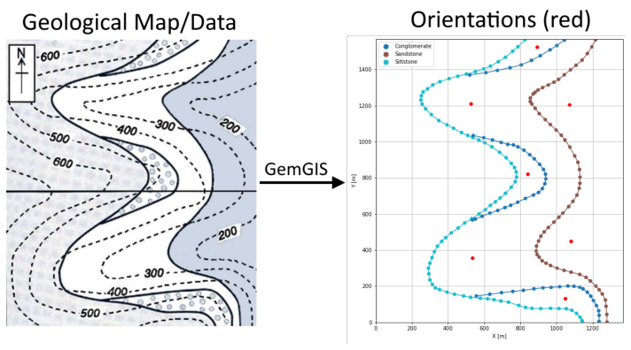
This example will show how to convert the geological map below using GemGIS to a GemPy model. This example is based on digitized data. The area is 1368 m wide (W-E extent) and 1568 m high (N-S extent). The model represents unconformable layers that dip to the west.
The map has been georeferenced with QGIS. The stratigraphic boundaries were digitized in QGIS. Strikes lines were digitized in QGIS as well and will be used to calculate orientations for the GemPy model. The contour lines were also digitized and will be interpolated with GemGIS to create a topography for the model.
Map Source: Unknown
[1]:
import matplotlib.pyplot as plt
import matplotlib.image as mpimg
img = mpimg.imread('../images/cover_example24.png')
plt.figure(figsize=(10, 10))
imgplot = plt.imshow(img)
plt.axis('off')
plt.tight_layout()
Licensing#
Computational Geosciences and Reservoir Engineering, RWTH Aachen University, Authors: Alexander Juestel. For more information contact: alexander.juestel(at)rwth-aachen.de
This work is licensed under a Creative Commons Attribution 4.0 International License (http://creativecommons.org/licenses/by/4.0/)
Import GemGIS#
If you have installed GemGIS via pip, you can import GemGIS like any other package. If you have downloaded the repository, append the path to the directory where the GemGIS repository is stored and then import GemGIS.
[2]:
import warnings
warnings.filterwarnings("ignore")
import gemgis as gg
Importing Libraries and loading Data#
All remaining packages can be loaded in order to prepare the data and to construct the model. The example data is downloaded form an external server using pooch. It will be stored in a data folder in the same directory where this notebook is stored.
[3]:
import geopandas as gpd
import rasterio
[4]:
file_path = 'data/example24/'
gg.download_gemgis_data.download_tutorial_data(filename="example24_unconformable_layers.zip", dirpath=file_path)
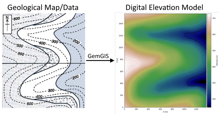
Creating Digital Elevation Model from Contour Lines#
The digital elevation model (DEM) will be created by interpolating contour lines digitized from the georeferenced map using the SciPy Radial Basis Function interpolation wrapped in GemGIS. The respective function used for that is gg.vector.interpolate_raster().
[5]:
import matplotlib.pyplot as plt
import matplotlib.image as mpimg
img = mpimg.imread('../images/dem_example24.png')
plt.figure(figsize=(10, 10))
imgplot = plt.imshow(img)
plt.axis('off')
plt.tight_layout()
[6]:
topo = gpd.read_file(file_path + 'topo24.shp')
topo.head()
[6]:
| id | Z | geometry | |
|---|---|---|---|
| 0 | None | 600 | LINESTRING (168.911 1471.213, 255.690 1480.424... |
| 1 | None | 500 | LINESTRING (174.728 1371.344, 230.965 1389.767... |
| 2 | None | 400 | LINESTRING (167.941 1287.474, 213.027 1305.412... |
| 3 | None | 200 | LINESTRING (1365.397 1329.167, 1332.915 1313.6... |
| 4 | None | 700 | LINESTRING (4.079 860.850, 49.165 845.821, 86.... |
Interpolating the contour lines#
[7]:
topo_raster = gg.vector.interpolate_raster(gdf=topo, value='Z', method='rbf', res=5)
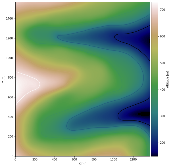
Plotting the raster#
[8]:
import matplotlib.pyplot as plt

from mpl_toolkits.axes_grid1 import make_axes_locatable

fix, ax = plt.subplots(1, figsize=(10,10))
topo.plot(ax=ax, aspect='equal', column='Z', cmap='gist_earth')
im = ax.imshow(topo_raster, origin='lower', extent=[0,1368,0,1568], cmap='gist_earth')
divider = make_axes_locatable(ax)
cax = divider.append_axes("right", size="5%", pad=0.05)
cbar = plt.colorbar(im, cax=cax)
cbar.set_label('Altitude [m]')
ax.set_xlabel('X [m]')
ax.set_ylabel('Y [m]')
[8]:
Text(95.40145646110935, 0.5, 'Y [m]')
Saving the raster to disc#
After the interpolation of the contour lines, the raster is saved to disc using gg.raster.save_as_tiff(). The function will not be executed as as raster is already provided with the example data.
Opening Raster#
The previously computed and saved raster can now be opened using rasterio.
[9]:
topo_raster = rasterio.open(file_path + 'raster24.tif')
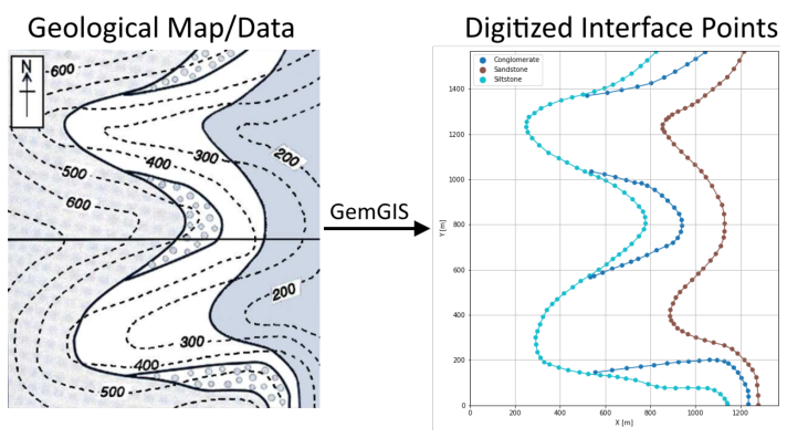
Interface Points of stratigraphic boundaries#
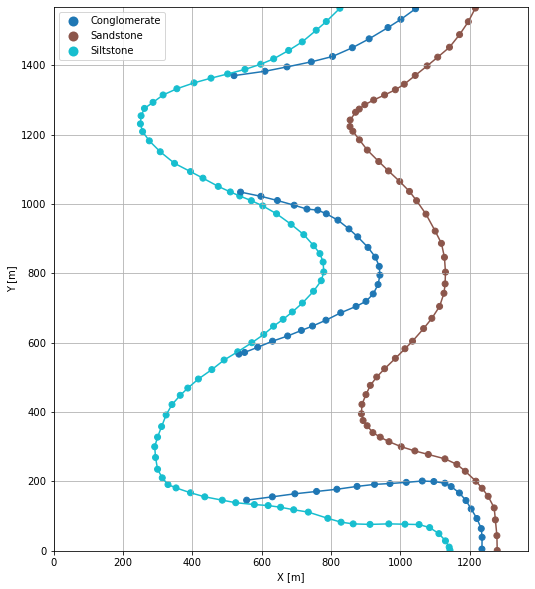
The interface points will be extracted from LineStrings digitized from the georeferenced map using QGIS. It is important to provide a formation name for each layer boundary. The vertical position of the interface point will be extracted from the digital elevation model using the GemGIS function gg.vector.extract_xyz(). The resulting GeoDataFrame now contains single points including the information about the respective formation.
[10]:
import matplotlib.pyplot as plt
import matplotlib.image as mpimg
img = mpimg.imread('../images/interfaces_example24.png')
plt.figure(figsize=(10, 10))
imgplot = plt.imshow(img)
plt.axis('off')
plt.tight_layout()
[11]:
interfaces = gpd.read_file(file_path + 'interfaces24.shp')
interfaces.head()
[11]:
| id | formation | geometry | |
|---|---|---|---|
| 0 | None | Conglomerate | LINESTRING (520.148 1370.617, 609.351 1383.222... |
| 1 | None | Conglomerate | LINESTRING (539.055 1034.651, 597.716 1022.531... |
| 2 | None | Conglomerate | LINESTRING (556.508 146.013, 630.683 155.709, ... |
| 3 | None | Siltstone | LINESTRING (825.572 1565.022, 786.303 1526.723... |
| 4 | None | Sandstone | LINESTRING (1216.321 1565.507, 1195.959 1526.2... |
Extracting XY coordinates from Digital Elevation Model#
[12]:
interfaces_coords = gg.vector.extract_xyz(gdf=interfaces, dem=topo_raster)
interfaces_coords = interfaces_coords.sort_values(by='formation', ascending=False)
interfaces_coords.head()
[12]:
| formation | geometry | X | Y | Z | |
|---|---|---|---|---|---|
| 99 | Siltstone | POINT (571.537 600.270) | 571.54 | 600.27 | 439.67 |
| 94 | Siltstone | POINT (717.462 714.683) | 717.46 | 714.68 | 494.31 |
| 88 | Siltstone | POINT (749.943 880.000) | 749.94 | 880.00 | 503.49 |
| 89 | Siltstone | POINT (767.881 857.214) | 767.88 | 857.21 | 504.65 |
| 90 | Siltstone | POINT (777.092 832.974) | 777.09 | 832.97 | 504.41 |
Plotting the Interface Points#
[13]:
fig, ax = plt.subplots(1, figsize=(10,10))

interfaces.plot(ax=ax, column='formation', legend=True, aspect='equal')
interfaces_coords.plot(ax=ax, column='formation', legend=True, aspect='equal')
plt.grid()
plt.xlabel('X [m]')
plt.ylabel('Y [m]')
plt.xlim(0,1368)
plt.ylim(0,1568)
[13]:
(0.0, 1568.0)
Orientations from Strike Lines#
Strike lines connect outcropping stratigraphic boundaries (interfaces) of the same altitude. In other words: the intersections between topographic contours and stratigraphic boundaries at the surface. The height difference and the horizontal difference between two digitized lines is used to calculate the dip and azimuth and hence an orientation that is necessary for GemPy. In order to calculate the orientations, each set of strikes lines/LineStrings for one formation must be given an id
number next to the altitude of the strike line. The id field is already predefined in QGIS. The strike line with the lowest altitude gets the id number 1, the strike line with the highest altitude the the number according to the number of digitized strike lines. It is currently recommended to use one set of strike lines for each structural element of one formation as illustrated.
[14]:
import matplotlib.pyplot as plt
import matplotlib.image as mpimg
img = mpimg.imread('../images/orientations_example24.png')
plt.figure(figsize=(10, 10))
imgplot = plt.imshow(img)
plt.axis('off')
plt.tight_layout()
[15]:
strikes = gpd.read_file(file_path + 'strikes24.shp')
strikes
[15]:
| id | formation | Z | geometry | |
|---|---|---|---|---|
| 0 | 1 | Sandstone2 | 300 | LINESTRING (998.646 566.334, 1000.100 300.179) |
| 1 | 1 | Sandstone1 | 300 | LINESTRING (987.980 1332.803, 987.980 1074.889) |
| 2 | 2 | Sandstone2 | 400 | LINESTRING (1161.539 249.275, 1158.630 686.564) |
| 3 | 2 | Sandstone1 | 400 | LINESTRING (1150.873 1463.699, 1154.267 953.689) |
| 4 | 1 | Siltstone2 | 400 | LINESTRING (313.623 1314.380, 314.593 1144.216) |
| 5 | 2 | Siltstone2 | 500 | LINESTRING (737.339 894.059, 742.671 1489.878) |
| 6 | 1 | Siltstone1 | 400 | LINESTRING (325.743 396.169, 328.167 190.129) |
| 7 | 2 | Siltstone1 | 500 | LINESTRING (736.369 737.468, 747.035 104.805) |
| 8 | 2 | Conglomerate2 | 500 | LINESTRING (875.022 883.878, 875.022 756.860) |
| 9 | 1 | Conglomerate2 | 500 | LINESTRING (803.271 886.787, 803.271 757.830) |
| 10 | 2 | Conglomerate3 | 500 | LINESTRING (937.076 1562.113, 936.591 1510.240) |
| 11 | 1 | Conglomerate3 | 500 | LINESTRING (848.843 1559.689, 848.843 1467.092) |
| 12 | 1 | Conglomerate1 | 500 | LINESTRING (1089.303 175.585, 1088.819 81.534) |
| 13 | 2 | Conglomerate1 | 500 | LINESTRING (1006.403 177.040, 1007.372 89.291) |
Calculate Orientations for each formation#
[16]:
orientations_sand1 = gg.vector.calculate_orientations_from_strike_lines(gdf=strikes[strikes['formation']=='Sandstone1'].sort_values(by='Z', ascending=True).reset_index())
orientations_sand1
[16]:
| dip | azimuth | Z | geometry | polarity | formation | X | Y | |
|---|---|---|---|---|---|---|---|---|
| 0 | 31.41 | 269.70 | 350.00 | POINT (1070.275 1206.270) | 1.00 | Sandstone1 | 1070.27 | 1206.27 |
[17]:
orientations_sand2 = gg.vector.calculate_orientations_from_strike_lines(gdf=strikes[strikes['formation']=='Sandstone2'].sort_values(by='Z', ascending=True).reset_index())
orientations_sand2
[17]:
| dip | azimuth | Z | geometry | polarity | formation | X | Y | |
|---|---|---|---|---|---|---|---|---|
| 0 | 31.88 | 269.64 | 350.00 | POINT (1079.729 450.588) | 1.00 | Sandstone2 | 1079.73 | 450.59 |
[18]:
orientations_silt1 = gg.vector.calculate_orientations_from_strike_lines(gdf=strikes[strikes['formation']=='Siltstone1'].sort_values(by='Z', ascending=True).reset_index())
orientations_silt1
[18]:
| dip | azimuth | Z | geometry | polarity | formation | X | Y | |
|---|---|---|---|---|---|---|---|---|
| 0 | 13.51 | 269.06 | 450.00 | POINT (534.329 357.143) | 1.00 | Siltstone1 | 534.33 | 357.14 |
[19]:
orientations_silt2 = gg.vector.calculate_orientations_from_strike_lines(gdf=strikes[strikes['formation']=='Siltstone2'].sort_values(by='Z', ascending=True).reset_index())
orientations_silt2
[19]:
| dip | azimuth | Z | geometry | polarity | formation | X | Y | |
|---|---|---|---|---|---|---|---|---|
| 0 | 13.24 | 270.45 | 450.00 | POINT (527.057 1210.633) | 1.00 | Siltstone2 | 527.06 | 1210.63 |
[20]:
orientations_conglomerate1 = gg.vector.calculate_orientations_from_strike_lines(gdf=strikes[strikes['formation']=='Conglomerate1'].sort_values(by='Z', ascending=True).reset_index())
orientations_conglomerate1
[20]:
| dip | azimuth | Z | geometry | polarity | formation | X | Y | |
|---|---|---|---|---|---|---|---|---|
| 0 | 0.00 | 0.00 | 500.00 | POINT (1047.974 130.863) | 1.00 | Conglomerate1 | 1047.97 | 130.86 |
[21]:
orientations_conglomerate2 = gg.vector.calculate_orientations_from_strike_lines(gdf=strikes[strikes['formation']=='Conglomerate2'].sort_values(by='Z', ascending=True).reset_index())
orientations_conglomerate2
[21]:
| dip | azimuth | Z | geometry | polarity | formation | X | Y | |
|---|---|---|---|---|---|---|---|---|
| 0 | 0.00 | 270.00 | 500.00 | POINT (839.147 821.339) | 1.00 | Conglomerate2 | 839.15 | 821.34 |
[22]:
orientations_conglomerate3 = gg.vector.calculate_orientations_from_strike_lines(gdf=strikes[strikes['formation']=='Conglomerate3'].sort_values(by='Z', ascending=True).reset_index())
orientations_conglomerate3
[22]:
| dip | azimuth | Z | geometry | polarity | formation | X | Y | |
|---|---|---|---|---|---|---|---|---|
| 0 | 0.00 | 90.54 | 500.00 | POINT (892.838 1524.784) | 1.00 | Conglomerate3 | 892.84 | 1524.78 |
Merging Orientations#
[23]:
import pandas as pd
orientations = pd.concat([orientations_sand1, orientations_sand2, orientations_silt1, orientations_silt2, orientations_conglomerate1, orientations_conglomerate2, orientations_conglomerate3]).reset_index()
orientations['formation'] = ['Sandstone', 'Sandstone', 'Siltstone', 'Siltstone', 'Conglomerate', 'Conglomerate', 'Conglomerate']
orientations
[23]:
| index | dip | azimuth | Z | geometry | polarity | formation | X | Y | |
|---|---|---|---|---|---|---|---|---|---|
| 0 | 0 | 31.41 | 269.70 | 350.00 | POINT (1070.275 1206.270) | 1.00 | Sandstone | 1070.27 | 1206.27 |
| 1 | 0 | 31.88 | 269.64 | 350.00 | POINT (1079.729 450.588) | 1.00 | Sandstone | 1079.73 | 450.59 |
| 2 | 0 | 13.51 | 269.06 | 450.00 | POINT (534.329 357.143) | 1.00 | Siltstone | 534.33 | 357.14 |
| 3 | 0 | 13.24 | 270.45 | 450.00 | POINT (527.057 1210.633) | 1.00 | Siltstone | 527.06 | 1210.63 |
| 4 | 0 | 0.00 | 0.00 | 500.00 | POINT (1047.974 130.863) | 1.00 | Conglomerate | 1047.97 | 130.86 |
| 5 | 0 | 0.00 | 270.00 | 500.00 | POINT (839.147 821.339) | 1.00 | Conglomerate | 839.15 | 821.34 |
| 6 | 0 | 0.00 | 90.54 | 500.00 | POINT (892.838 1524.784) | 1.00 | Conglomerate | 892.84 | 1524.78 |
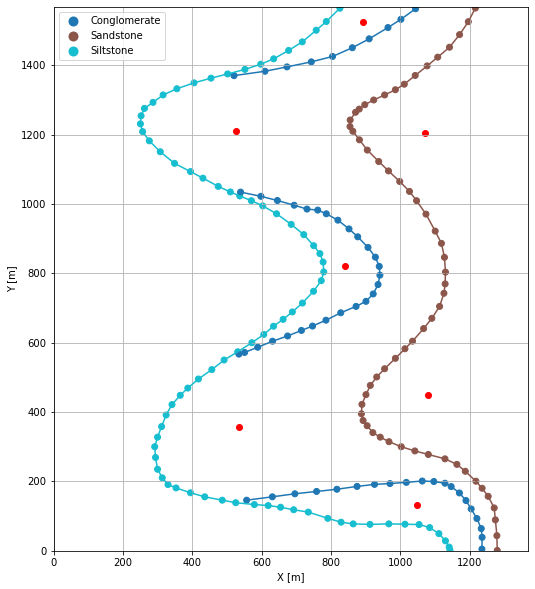
Plotting the Orientations#
[24]:
fig, ax = plt.subplots(1, figsize=(10,10))

interfaces.plot(ax=ax, column='formation', legend=True, aspect='equal')
interfaces_coords.plot(ax=ax, column='formation', legend=True, aspect='equal')
orientations.plot(ax=ax, color='red', aspect='equal')
plt.grid()
plt.xlabel('X [m]')
plt.ylabel('Y [m]')
plt.xlim(0,1368)
plt.ylim(0,1568)
[24]:
(0.0, 1568.0)
GemPy Model Construction#
The structural geological model will be constructed using the GemPy package.
[25]:
import gempy as gp
WARNING (theano.configdefaults): g++ not available, if using conda: `conda install m2w64-toolchain`
WARNING (theano.configdefaults): g++ not detected ! Theano will be unable to execute optimized C-implementations (for both CPU and GPU) and will default to Python implementations. Performance will be severely degraded. To remove this warning, set Theano flags cxx to an empty string.
WARNING (theano.tensor.blas): Using NumPy C-API based implementation for BLAS functions.
Creating new Model#
[26]:
geo_model = gp.create_model('Model24')
geo_model
[26]:
Model24 2022-04-08 08:28
Initiate Data#
[27]:
gp.init_data(geo_model, [0,1368,0,1568,0,800], [100,100,100],
             surface_points_df = interfaces_coords[interfaces_coords['Z']!=0],
             orientations_df = orientations,
             default_values=True)
Active grids: ['regular']
[27]:
Model24 2022-04-08 08:28
Model Surfaces#
[28]:
geo_model.surfaces
[28]:
| surface | series | order_surfaces | color | id | |
|---|---|---|---|---|---|
| 0 | Siltstone | Default series | 1 | #015482 | 1 |
| 1 | Sandstone | Default series | 2 | #9f0052 | 2 |
| 2 | Conglomerate | Default series | 3 | #ffbe00 | 3 |
Mapping the Stack to Surfaces#
[29]:
gp.map_stack_to_surfaces(geo_model,
                         {
                          'Strata1': ('Siltstone'),
                          'Strata2': ('Conglomerate'),
                          'Strata3': ('Sandstone'),
                         },
                         remove_unused_series=True)
geo_model.add_surfaces('Claystone')
[29]:
| surface | series | order_surfaces | color | id | |
|---|---|---|---|---|---|
| 0 | Siltstone | Strata1 | 1 | #015482 | 1 |
| 2 | Conglomerate | Strata2 | 1 | #9f0052 | 2 |
| 1 | Sandstone | Strata3 | 1 | #ffbe00 | 3 |
| 3 | Claystone | Strata3 | 2 | #728f02 | 4 |
Adding additional Orientations#
[30]:
geo_model.add_orientations(X=600, Y=50, Z=400, surface='Conglomerate', orientation = [0,0,1])
geo_model.add_orientations(X=150, Y=50, Z=400, surface='Conglomerate', orientation = [0,0,1])
geo_model.add_orientations(X=600, Y=275, Z=400, surface='Conglomerate', orientation = [0,0,1])
geo_model.add_orientations(X=150, Y=275, Z=400, surface='Conglomerate', orientation = [0,0,1])
geo_model.add_orientations(X=600, Y=850, Z=400, surface='Conglomerate', orientation = [0,0,1])
geo_model.add_orientations(X=150, Y=850, Z=400, surface='Conglomerate', orientation = [0,0,1])
geo_model.add_orientations(X=600, Y=1250, Z=400, surface='Conglomerate', orientation = [0,0,1])
geo_model.add_orientations(X=150, Y=1250, Z=400, surface='Conglomerate', orientation = [0,0,1])
geo_model.add_orientations(X=600, Y=1500, Z=400, surface='Conglomerate', orientation = [0,0,1])
geo_model.add_orientations(X=150, Y=1500, Z=400, surface='Conglomerate', orientation = [0,0,1])

geo_model.add_orientations(X=600, Y=50, Z=500, surface='Siltstone', orientation = [270,13.5,1])
geo_model.add_orientations(X=150, Y=50, Z=500, surface='Siltstone', orientation = [270,13.5,1])
geo_model.add_orientations(X=600, Y=275, Z=500, surface='Siltstone', orientation = [270,13.5,1])
geo_model.add_orientations(X=150, Y=275, Z=500, surface='Siltstone', orientation = [270,13.5,1])
geo_model.add_orientations(X=600, Y=850, Z=500, surface='Siltstone', orientation = [270,13.5,1])
geo_model.add_orientations(X=150, Y=850, Z=500, surface='Siltstone', orientation = [270,13.5,1])
geo_model.add_orientations(X=600, Y=1250, Z=500, surface='Siltstone', orientation = [270,13.5,1])
geo_model.add_orientations(X=150, Y=1250, Z=500, surface='Siltstone', orientation = [270,13.5,1])
geo_model.add_orientations(X=600, Y=1500, Z=500, surface='Siltstone', orientation = [270,13.5,1])
geo_model.add_orientations(X=150, Y=1500, Z=500, surface='Siltstone', orientation = [270,13.5,1])

geo_model.add_orientations(X=600, Y=50, Z=300, surface='Sandstone', orientation = [270,31.5,1])
geo_model.add_orientations(X=150, Y=50, Z=300, surface='Sandstone', orientation = [270,31.5,1])
geo_model.add_orientations(X=600, Y=275, Z=300, surface='Sandstone', orientation = [270,31.5,1])
geo_model.add_orientations(X=150, Y=275, Z=300, surface='Sandstone', orientation = [270,31.5,1])
geo_model.add_orientations(X=600, Y=850, Z=300, surface='Sandstone', orientation = [270,31.5,1])
geo_model.add_orientations(X=150, Y=850, Z=300, surface='Sandstone', orientation = [270,31.5,1])
geo_model.add_orientations(X=600, Y=1250, Z=300, surface='Sandstone', orientation = [270,31.5,1])
geo_model.add_orientations(X=150, Y=1250, Z=300, surface='Sandstone', orientation = [270,31.5,1])
geo_model.add_orientations(X=600, Y=1500, Z=300, surface='Sandstone', orientation = [270,31.5,1])
geo_model.add_orientations(X=150, Y=1500, Z=300, surface='Sandstone', orientation = [270,31.5,1])
[30]:
| X | Y | Z | G_x | G_y | G_z | smooth | surface | |
|---|---|---|---|---|---|---|---|---|
| 2 | 534.33 | 357.14 | 450.00 | -0.23 | -0.00 | 0.97 | 0.01 | Siltstone |
| 3 | 527.06 | 1210.63 | 450.00 | -0.23 | 0.00 | 0.97 | 0.01 | Siltstone |
| 17 | 600.00 | 50.00 | 500.00 | -0.23 | 0.00 | 0.97 | 0.01 | Siltstone |
| 18 | 150.00 | 50.00 | 500.00 | -0.23 | 0.00 | 0.97 | 0.01 | Siltstone |
| 19 | 600.00 | 275.00 | 500.00 | -0.23 | 0.00 | 0.97 | 0.01 | Siltstone |
| 20 | 150.00 | 275.00 | 500.00 | -0.23 | 0.00 | 0.97 | 0.01 | Siltstone |
| 21 | 600.00 | 850.00 | 500.00 | -0.23 | 0.00 | 0.97 | 0.01 | Siltstone |
| 22 | 150.00 | 850.00 | 500.00 | -0.23 | 0.00 | 0.97 | 0.01 | Siltstone |
| 23 | 600.00 | 1250.00 | 500.00 | -0.23 | 0.00 | 0.97 | 0.01 | Siltstone |
| 24 | 150.00 | 1250.00 | 500.00 | -0.23 | 0.00 | 0.97 | 0.01 | Siltstone |
| 25 | 600.00 | 1500.00 | 500.00 | -0.23 | 0.00 | 0.97 | 0.01 | Siltstone |
| 26 | 150.00 | 1500.00 | 500.00 | -0.23 | 0.00 | 0.97 | 0.01 | Siltstone |
| 4 | 1047.97 | 130.86 | 500.00 | 0.00 | 0.00 | 1.00 | 0.01 | Conglomerate |
| 5 | 839.15 | 821.34 | 500.00 | 0.00 | 0.00 | 1.00 | 0.01 | Conglomerate |
| 6 | 892.84 | 1524.78 | 500.00 | 0.00 | 0.00 | 1.00 | 0.01 | Conglomerate |
| 7 | 600.00 | 50.00 | 400.00 | 0.00 | 0.00 | 1.00 | 0.01 | Conglomerate |
| 8 | 150.00 | 50.00 | 400.00 | 0.00 | 0.00 | 1.00 | 0.01 | Conglomerate |
| 9 | 600.00 | 275.00 | 400.00 | 0.00 | 0.00 | 1.00 | 0.01 | Conglomerate |
| 10 | 150.00 | 275.00 | 400.00 | 0.00 | 0.00 | 1.00 | 0.01 | Conglomerate |
| 11 | 600.00 | 850.00 | 400.00 | 0.00 | 0.00 | 1.00 | 0.01 | Conglomerate |
| 12 | 150.00 | 850.00 | 400.00 | 0.00 | 0.00 | 1.00 | 0.01 | Conglomerate |
| 13 | 600.00 | 1250.00 | 400.00 | 0.00 | 0.00 | 1.00 | 0.01 | Conglomerate |
| 14 | 150.00 | 1250.00 | 400.00 | 0.00 | 0.00 | 1.00 | 0.01 | Conglomerate |
| 15 | 600.00 | 1500.00 | 400.00 | 0.00 | 0.00 | 1.00 | 0.01 | Conglomerate |
| 16 | 150.00 | 1500.00 | 400.00 | 0.00 | 0.00 | 1.00 | 0.01 | Conglomerate |
| 0 | 1070.27 | 1206.27 | 350.00 | -0.52 | -0.00 | 0.85 | 0.01 | Sandstone |
| 1 | 1079.73 | 450.59 | 350.00 | -0.53 | -0.00 | 0.85 | 0.01 | Sandstone |
| 27 | 600.00 | 50.00 | 300.00 | -0.52 | 0.00 | 0.85 | 0.01 | Sandstone |
| 28 | 150.00 | 50.00 | 300.00 | -0.52 | 0.00 | 0.85 | 0.01 | Sandstone |
| 29 | 600.00 | 275.00 | 300.00 | -0.52 | 0.00 | 0.85 | 0.01 | Sandstone |
| 30 | 150.00 | 275.00 | 300.00 | -0.52 | 0.00 | 0.85 | 0.01 | Sandstone |
| 31 | 600.00 | 850.00 | 300.00 | -0.52 | 0.00 | 0.85 | 0.01 | Sandstone |
| 32 | 150.00 | 850.00 | 300.00 | -0.52 | 0.00 | 0.85 | 0.01 | Sandstone |
| 33 | 600.00 | 1250.00 | 300.00 | -0.52 | 0.00 | 0.85 | 0.01 | Sandstone |
| 34 | 150.00 | 1250.00 | 300.00 | -0.52 | 0.00 | 0.85 | 0.01 | Sandstone |
| 35 | 600.00 | 1500.00 | 300.00 | -0.52 | 0.00 | 0.85 | 0.01 | Sandstone |
| 36 | 150.00 | 1500.00 | 300.00 | -0.52 | 0.00 | 0.85 | 0.01 | Sandstone |
Showing the Number of Data Points#
[31]:
gg.utils.show_number_of_data_points(geo_model=geo_model)
[31]:
| surface | series | order_surfaces | color | id | No. of Interfaces | No. of Orientations | |
|---|---|---|---|---|---|---|---|
| 0 | Siltstone | Strata1 | 1 | #015482 | 1 | 80 | 12 |
| 2 | Conglomerate | Strata2 | 1 | #9f0052 | 2 | 57 | 13 |
| 1 | Sandstone | Strata3 | 1 | #ffbe00 | 3 | 61 | 12 |
| 3 | Claystone | Strata3 | 2 | #728f02 | 4 | 0 | 0 |
Loading Digital Elevation Model#
[32]:
geo_model.set_topography(
    source='gdal', filepath=file_path + 'raster24.tif')
Cropped raster to geo_model.grid.extent.
depending on the size of the raster, this can take a while...
storing converted file...
Active grids: ['regular' 'topography']
[32]:
Grid Object. Values:
array([[   6.84      ,    7.84      ,    4.        ],
       [   6.84      ,    7.84      ,   12.        ],
       [   6.84      ,    7.84      ,   20.        ],
       ...,
       [1365.49450549, 1555.47603834,  383.11444092],
       [1365.49450549, 1560.485623  ,  386.23483276],
       [1365.49450549, 1565.49520767,  389.29962158]])
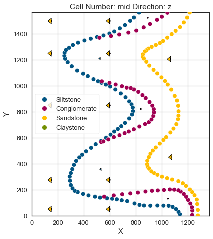
Plotting Input Data#
[33]:
gp.plot_2d(geo_model, direction='z', show_lith=False, show_boundaries=False)
plt.grid()
[34]:
gp.plot_3d(geo_model, image=False, plotter_type='basic', notebook=True)
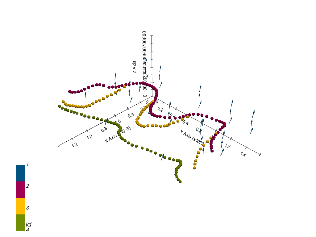
[34]:
<gempy.plot.vista.GemPyToVista at 0x20f8cfe3340>
Setting the Interpolator#
[35]:
gp.set_interpolator(geo_model,
                    compile_theano=True,
                    theano_optimizer='fast_compile',
                    verbose=[],
                    update_kriging = False
                    )
Compiling theano function...
Level of Optimization:  fast_compile
Device:  cpu
Precision:  float64
Number of faults:  0
Compilation Done!
Kriging values:
                     values
range              2229.36
$C_o$            118334.48
drift equations  [3, 3, 3]
[35]:
<gempy.core.interpolator.InterpolatorModel at 0x20f86f139d0>
Computing Model#
[36]:
sol = gp.compute_model(geo_model, compute_mesh=True)
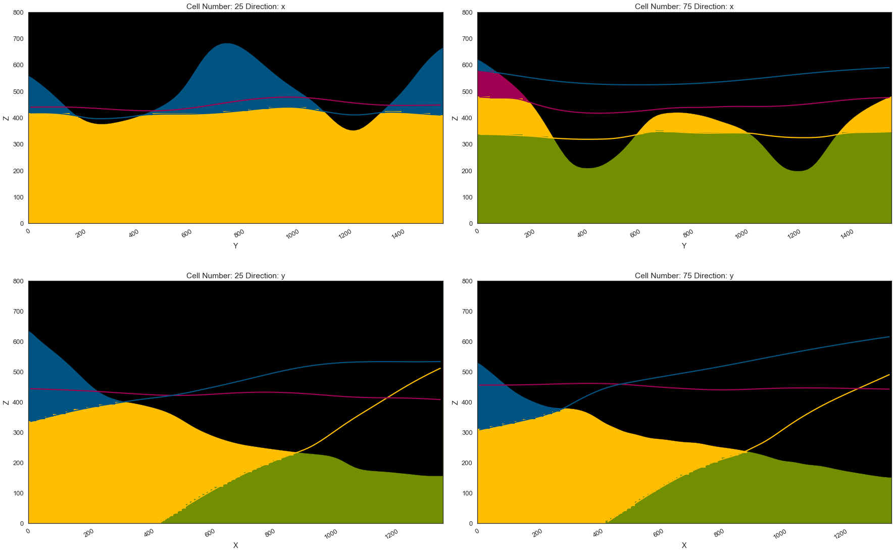
Plotting Cross Sections#
[37]:
gp.plot_2d(geo_model, direction=['x', 'x', 'y', 'y'], cell_number=[25,75,25,75], show_topography=True, show_data=False)
[37]:
<gempy.plot.visualization_2d.Plot2D at 0x20f8b580220>
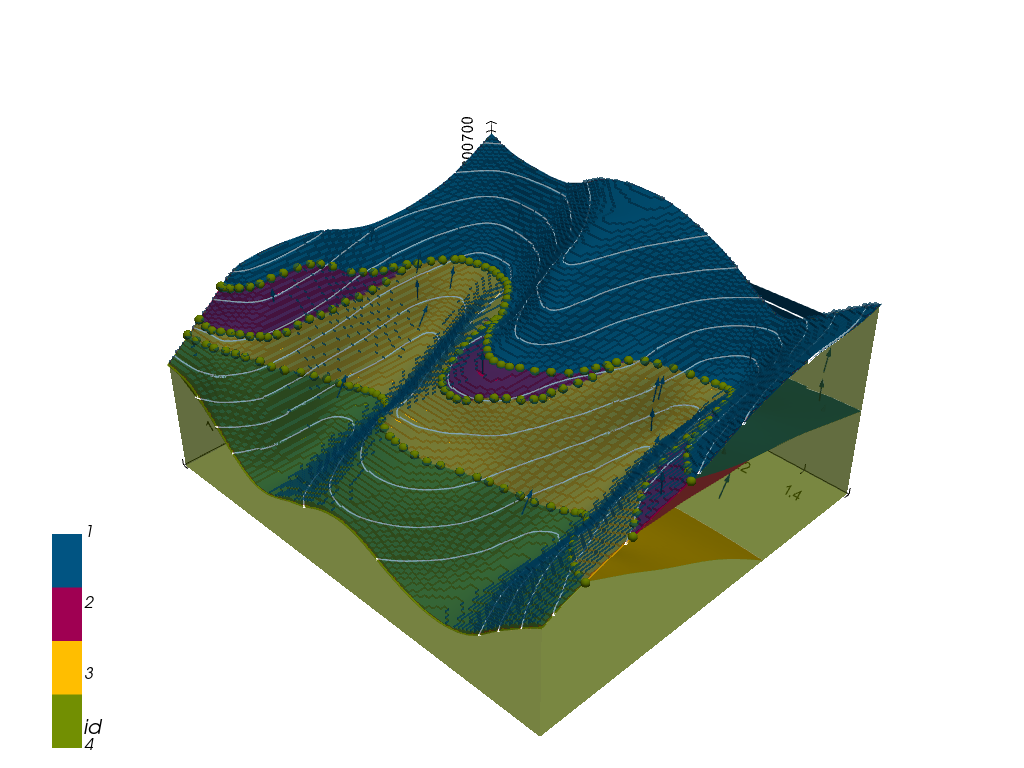
Plotting 3D Model#
[38]:
gpv = gp.plot_3d(geo_model, image=False, show_topography=True,
                 plotter_type='basic', notebook=True, show_lith=True)
[ ]: