
Example 31 - Folded Layers
Contents
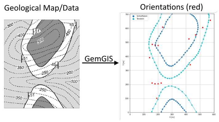
Example 31 - Folded Layers#
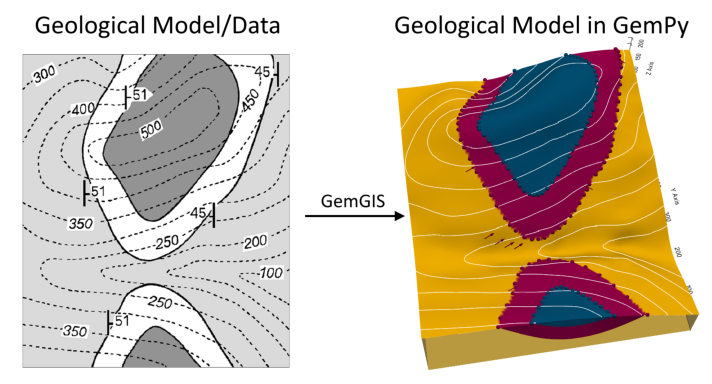
This example will show how to convert the geological map below using GemGIS to a GemPy model. This example is based on digitized data. The area is 601 m wide (W-E extent) and 705 m high (N-S extent). The vertical model extents varies between 0 m and 300 m. The model represents two folded stratigraphic units (blue and red) above an unspecified basement (yellow). The map has been georeferenced with QGIS. The stratigraphic boundaries were digitized in QGIS. Strikes lines were digitized in
QGIS as well and were used to calculate orientations for the GemPy model. These will be loaded into the model directly. The contour lines were also digitized and will be interpolated with GemGIS to create a topography for the model.
Map Source: Unknown
[1]:
import matplotlib.pyplot as plt
import matplotlib.image as mpimg
img = mpimg.imread('../images/cover_example31.png')
plt.figure(figsize=(10, 10))
imgplot = plt.imshow(img)
plt.axis('off')
plt.tight_layout()
Licensing#
Computational Geosciences and Reservoir Engineering, RWTH Aachen University, Authors: Alexander Juestel. For more information contact: alexander.juestel(at)rwth-aachen.de
This work is licensed under a Creative Commons Attribution 4.0 International License (http://creativecommons.org/licenses/by/4.0/)
Import GemGIS#
If you have installed GemGIS via pip or conda, you can import GemGIS like any other package. If you have downloaded the repository, append the path to the directory where the GemGIS repository is stored and then import GemGIS.
[2]:
import warnings
warnings.filterwarnings("ignore")
import gemgis as gg
Importing Libraries and loading Data#
All remaining packages can be loaded in order to prepare the data and to construct the model. The example data is downloaded from an external server using pooch. It will be stored in a data folder in the same directory where this notebook is stored.
[3]:
import geopandas as gpd
import rasterio
[4]:
file_path = 'data/example31/'
gg.download_gemgis_data.download_tutorial_data(filename="example31_folded_layers.zip", dirpath=file_path)
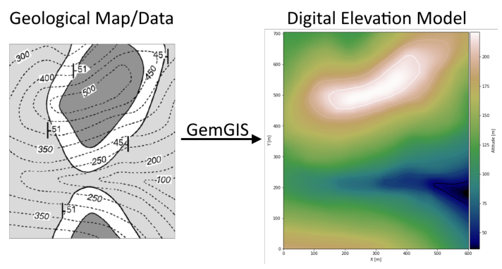
Creating Digital Elevation Model from Contour Lines#
The digital elevation model (DEM) will be created by interpolating contour lines digitized from the georeferenced map using the SciPy Radial Basis Function interpolation wrapped in GemGIS. The respective function used for that is gg.vector.interpolate_raster().
[5]:
img = mpimg.imread('../images/dem_example31.png')
plt.figure(figsize=(10, 10))
imgplot = plt.imshow(img)
plt.axis('off')
plt.tight_layout()
[6]:
topo = gpd.read_file(file_path + 'topo31.shp')
topo['Z'] = topo['Z']*0.425
topo.head()
[6]:
| id | Z | geometry | |
|---|---|---|---|
| 0 | None | 170.00 | LINESTRING (0.994 52.851, 36.954 48.266, 68.32... |
| 1 | None | 148.75 | LINESTRING (1.235 98.706, 42.022 94.603, 80.39... |
| 2 | None | 127.50 | LINESTRING (1.477 157.955, 44.435 147.818, 81.... |
| 3 | None | 127.50 | LINESTRING (1.597 320.738, 11.492 310.722, 22.... |
| 4 | None | 106.25 | LINESTRING (553.299 3.497, 534.233 30.527, 513... |
Interpolating the contour lines#
[7]:
topo_raster = gg.vector.interpolate_raster(gdf=topo, value='Z', method='rbf', res=5)
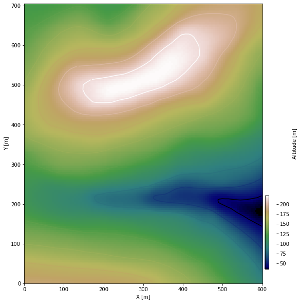
Plotting the raster#
[8]:
import matplotlib.pyplot as plt

from mpl_toolkits.axes_grid1 import make_axes_locatable

fig, ax = plt.subplots(1, figsize=(10, 10))
topo.plot(ax=ax, aspect='equal', column='Z', cmap='gist_earth')
im = ax.imshow(topo_raster, origin='lower', extent=[0, 601, 0, 705], cmap='gist_earth')
divider = make_axes_locatable(ax)
cax = divider.append_axes("right", size="5%", pad=0.05)
cbar = plt.colorbar(im, cax=cax)
cbar.set_label('Altitude [m]')
ax.set_xlabel('X [m]')
ax.set_ylabel('Y [m]')
plt.xlim(0, 601)
plt.ylim(0, 705)
[8]:
(0.0, 705.0)
Saving the raster to disc#
After the interpolation of the contour lines, the raster is saved to disc using gg.raster.save_as_tiff(). The function will not be executed as a raster is already provided with the example data.
Opening Raster#
The previously computed and saved raster can now be opened using rasterio.
[9]:
topo_raster = rasterio.open(file_path + 'raster31.tif')
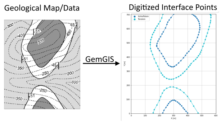
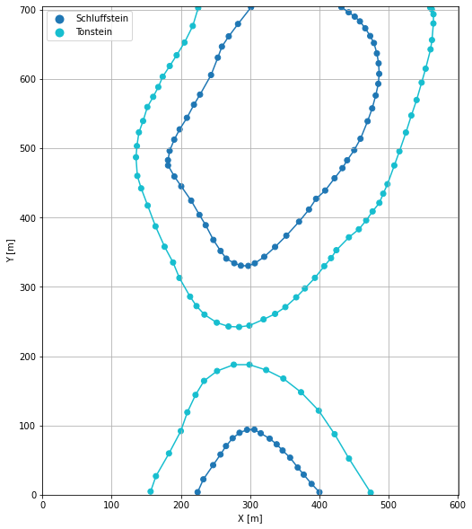
Interface Points of stratigraphic boundaries#
The interface points will be extracted from LineStrings digitized from the georeferenced map using QGIS. It is important to provide a formation name for each layer boundary. The vertical position of the interface point will be extracted from the digital elevation model using the GemGIS function gg.vector.extract_xyz(). The resulting GeoDataFrame now contains single points including the information about the respective formation.
[10]:
img = mpimg.imread('../images/interfaces_example31.png')
plt.figure(figsize=(10, 10))
imgplot = plt.imshow(img)
plt.axis('off')
plt.tight_layout()
[11]:
interfaces = gpd.read_file(file_path + 'interfaces31.shp')
interfaces.head()
[11]:
| id | formation | geometry | |
|---|---|---|---|
| 0 | None | Schluffstein | LINESTRING (224.233 3.618, 232.559 22.201, 246... |
| 1 | None | Tonstein | LINESTRING (156.296 4.583, 164.019 26.787, 182... |
| 2 | None | Tonstein | LINESTRING (225.078 702.899, 217.234 676.834, ... |
| 3 | None | Schluffstein | LINESTRING (301.462 703.864, 282.637 679.730, ... |
Extracting Z coordinate from Digital Elevation Model#
[12]:
interfaces_coords = gg.vector.extract_xyz(gdf=interfaces, dem=topo_raster)
interfaces_coords = interfaces_coords[interfaces_coords['formation'].isin(['Tonstein', 'Schluffstein'])]
interfaces_coords
[12]:
| formation | geometry | X | Y | Z | |
|---|---|---|---|---|---|
| 0 | Schluffstein | POINT (224.233 3.618) | 224.23 | 3.62 | 180.40 |
| 1 | Schluffstein | POINT (232.559 22.201) | 232.56 | 22.20 | 172.51 |
| 2 | Schluffstein | POINT (246.677 42.715) | 246.68 | 42.72 | 161.16 |
| 3 | Schluffstein | POINT (257.296 58.040) | 257.30 | 58.04 | 151.99 |
| 4 | Schluffstein | POINT (265.261 70.228) | 265.26 | 70.23 | 144.44 |
| ... | ... | ... | ... | ... | ... |
| 138 | Schluffstein | POINT (466.538 673.456) | 466.54 | 673.46 | 193.52 |
| 139 | Schluffstein | POINT (458.815 683.471) | 458.81 | 683.47 | 189.84 |
| 140 | Schluffstein | POINT (451.333 690.349) | 451.33 | 690.35 | 186.16 |
| 141 | Schluffstein | POINT (442.524 696.624) | 442.52 | 696.62 | 183.49 |
| 142 | Schluffstein | POINT (432.026 704.106) | 432.03 | 704.11 | 180.41 |
143 rows × 5 columns
Plotting the Interface Points#
[13]:
fig, ax = plt.subplots(1, figsize=(10, 10))

interfaces.plot(ax=ax, column='formation', legend=True, aspect='equal')
interfaces_coords.plot(ax=ax, column='formation', legend=True, aspect='equal')
plt.grid()
plt.xlabel('X [m]')
plt.ylabel('Y [m]')
plt.xlim(0, 601)
plt.ylim(0, 705)
[13]:
(0.0, 705.0)
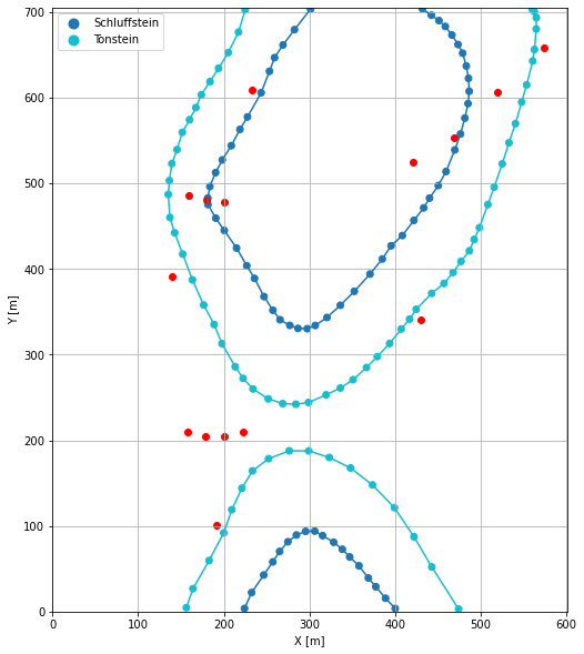
Orientations from Strike Lines and Map#
Strike lines connect outcropping stratigraphic boundaries (interfaces) of the same altitude. In other words: the intersections between topographic contours and stratigraphic boundaries at the surface. The height difference and the horizontal difference between two digitized lines is used to calculate the dip and azimuth and hence an orientation that is necessary for GemPy. In order to calculate the orientations, each set of strikes lines/LineStrings for one formation must be given an id
number next to the altitude of the strike line. The id field is already predefined in QGIS. The strike line with the lowest altitude gets the id number 1, the strike line with the highest altitude the the number according to the number of digitized strike lines. It is currently recommended to use one set of strike lines for each structural element of one formation as illustrated.
In addition, orientations were provided on the map which were digitized as points and can be used right away.
[14]:
img = mpimg.imread('../images/orientations_example31.png')
plt.figure(figsize=(10, 10))
imgplot = plt.imshow(img)
plt.axis('off')
plt.tight_layout()
Orientations from Map#
[15]:
orientations_points = gpd.read_file(file_path + 'orientations31.shp')
orientations_points = gg.vector.extract_xyz(gdf=orientations_points, dem=topo_raster)
orientations_points
[15]:
| formation | dip | azimuth | polarity | geometry | X | Y | Z | |
|---|---|---|---|---|---|---|---|---|
| 0 | Tonstein | 51.00 | 90.00 | 1.00 | POINT (139.161 391.089) | 139.16 | 391.09 | 175.58 |
| 1 | Tonstein | 45.00 | 270.00 | 1.00 | POINT (430.216 340.890) | 430.22 | 340.89 | 112.43 |
| 2 | Tonstein | 51.00 | 90.00 | 1.00 | POINT (192.014 101.481) | 192.01 | 101.48 | 136.37 |
| 3 | Tonstein | 51.00 | 90.00 | 1.00 | POINT (232.559 608.777) | 232.56 | 608.78 | 160.57 |
| 4 | Tonstein | 45.00 | 270.00 | 1.00 | POINT (574.296 658.493) | 574.30 | 658.49 | 179.60 |
Orientations from Strike Lines#
[16]:
strikes = gpd.read_file(file_path + 'strikes31.shp')
strikes['Z'] = strikes['Z']*0.425
strikes
[16]:
| id | formation | Z | geometry | |
|---|---|---|---|---|
| 0 | 1 | Tonstein | 106.25 | LINESTRING (234.450 260.524, 234.691 164.713) |
| 1 | 2 | Tonstein | 127.50 | LINESTRING (210.799 289.485, 210.799 124.168) |
| 2 | 3 | Tonstein | 148.75 | LINESTRING (190.044 331.719, 190.044 74.934) |
| 3 | 4 | Tonstein | 170.00 | LINESTRING (168.564 374.919, 168.082 36.561) |
| 4 | 5 | Tonstein | 191.25 | LINESTRING (148.533 425.842, 143.465 3.498) |
| 5 | 4 | Tonstein1 | 191.25 | LINESTRING (148.775 425.600, 149.499 550.132) |
| 6 | 3 | Tonstein1 | 170.00 | LINESTRING (169.288 592.849, 168.806 374.437) |
| 7 | 2 | Tonstein1 | 148.75 | LINESTRING (190.285 628.326, 190.285 330.513) |
| 8 | 1 | Tonstein1 | 127.50 | LINESTRING (210.558 663.561, 211.040 289.968) |
| 9 | 1 | Schluffstein5 | 148.75 | LINESTRING (261.239 62.867, 257.860 350.544) |
| 10 | 2 | Schluffstein5 | 170.00 | LINESTRING (237.105 28.356, 235.898 386.504) |
| 11 | 1 | Schluffstein4 | 148.75 | LINESTRING (364.291 42.836, 365.739 390.365) |
| 12 | 3 | Schluffstein5 | 191.25 | LINESTRING (213.695 425.600, 215.143 2.291) |
| 13 | 4 | Schluffstein5 | 212.50 | LINESTRING (191.974 456.009, 193.422 4.705) |
| 14 | 2 | Schluffstein4 | 170.00 | LINESTRING (421.247 453.113, 423.178 2.774) |
| 15 | 3 | Schluffstein4 | 191.25 | LINESTRING (463.240 520.206, 463.240 0.843) |
| 16 | 4 | Schluffstein1 | 212.50 | LINESTRING (192.457 516.827, 191.974 454.803) |
| 17 | 3 | Schluffstein1 | 191.25 | LINESTRING (214.902 555.200, 213.695 425.600) |
| 18 | 2 | Schluffstein1 | 170.00 | LINESTRING (237.588 595.021, 235.657 387.710) |
| 19 | 1 | Schluffstein1 | 148.75 | LINESTRING (257.136 640.875, 257.136 349.579) |
| 20 | 3 | Schluffstein2 | 191.25 | LINESTRING (461.309 679.972, 463.240 520.447) |
| 21 | 2 | Schluffstein2 | 170.00 | LINESTRING (421.005 454.079, 419.557 701.934) |
| 22 | 1 | Schluffstein2 | 148.75 | LINESTRING (365.739 390.365, 364.773 703.865) |
| 23 | 1 | Schluffstein3 | 148.75 | LINESTRING (257.136 640.151, 258.101 351.027) |
| 24 | 2 | Schluffstein3 | 148.75 | LINESTRING (365.256 389.158, 364.773 703.865) |
| 25 | 4 | Tonstein2 | 170.00 | LINESTRING (542.882 580.058, 544.813 705.072) |
| 26 | 3 | Tonstein2 | 148.75 | LINESTRING (493.649 436.702, 495.579 703.624) |
| 27 | 2 | Tonstein2 | 127.50 | LINESTRING (443.933 371.540, 444.898 703.624) |
| 28 | 1 | Tonstein2 | 106.25 | LINESTRING (399.044 319.411, 397.596 704.589) |
Calculating Orientations for each formation#
[17]:
orientations_claystone1 = gg.vector.calculate_orientations_from_strike_lines(gdf=strikes[strikes['formation'] == 'Tonstein1'].sort_values(by='id', ascending=True).reset_index())
orientations_claystone1
[17]:
| dip | azimuth | Z | geometry | polarity | formation | X | Y | |
|---|---|---|---|---|---|---|---|---|
| 0 | 46.28 | 89.95 | 138.12 | POINT (200.542 478.092) | 1.00 | Tonstein1 | 200.54 | 478.09 |
| 1 | 45.34 | 90.04 | 159.38 | POINT (179.666 481.531) | 1.00 | Tonstein1 | 179.67 | 481.53 |
| 2 | 47.17 | 90.18 | 180.62 | POINT (159.092 485.754) | 1.00 | Tonstein1 | 159.09 | 485.75 |
[18]:
orientations_claystone = gg.vector.calculate_orientations_from_strike_lines(gdf=strikes[strikes['formation'] == 'Tonstein'].sort_values(by='id', ascending=True).reset_index())
orientations_claystone
[18]:
| dip | azimuth | Z | geometry | polarity | formation | X | Y | |
|---|---|---|---|---|---|---|---|---|
| 0 | 41.94 | 89.96 | 116.88 | POINT (222.685 209.722) | 1.00 | Tonstein | 222.68 | 209.72 |
| 1 | 45.67 | 90.00 | 138.12 | POINT (200.421 205.077) | 1.00 | Tonstein | 200.42 | 205.08 |
| 2 | 44.61 | 90.05 | 159.38 | POINT (179.183 204.534) | 1.00 | Tonstein | 179.18 | 204.53 |
| 3 | 45.83 | 90.45 | 180.62 | POINT (157.161 210.205) | 1.00 | Tonstein | 157.16 | 210.21 |
[19]:
orientations_claystone2 = gg.vector.calculate_orientations_from_strike_lines(gdf=strikes[strikes['formation'] == 'Tonstein2'].sort_values(by='id', ascending=True).reset_index())
orientations_claystone2
[19]:
| dip | azimuth | Z | geometry | polarity | formation | X | Y | |
|---|---|---|---|---|---|---|---|---|
| 0 | 25.24 | 269.95 | 116.88 | POINT (421.368 524.791) | 1.00 | Tonstein2 | 421.37 | 524.79 |
| 1 | 23.22 | 270.26 | 138.12 | POINT (469.515 553.872) | 1.00 | Tonstein2 | 469.51 | 553.87 |
| 2 | 23.79 | 270.50 | 159.38 | POINT (519.231 606.364) | 1.00 | Tonstein2 | 519.23 | 606.36 |
[20]:
orientations_siltstone1 = gg.vector.calculate_orientations_from_strike_lines(gdf=strikes[strikes['formation'] == 'Schluffstein1'].sort_values(by='id', ascending=True).reset_index())
orientations_siltstone1
[20]:
| dip | azimuth | Z | geometry | polarity | formation | X | Y | |
|---|---|---|---|---|---|---|---|---|
| 0 | 47.39 | 90.18 | 159.38 | POINT (246.879 493.296) | 1.00 | Schluffstein1 | 246.88 | 493.30 |
| 1 | 43.60 | 90.53 | 180.62 | POINT (225.460 490.883) | 1.00 | Schluffstein1 | 225.46 | 490.88 |
| 2 | 44.02 | 90.52 | 201.88 | POINT (203.257 488.107) | 1.00 | Schluffstein1 | 203.26 | 488.11 |
[21]:
orientations_siltstone2 = gg.vector.calculate_orientations_from_strike_lines(gdf=strikes[strikes['formation'] == 'Schluffstein2'].sort_values(by='id', ascending=True).reset_index())
orientations_siltstone2
[21]:
| dip | azimuth | Z | geometry | polarity | formation | X | Y | |
|---|---|---|---|---|---|---|---|---|
| 0 | 21.20 | 269.76 | 159.38 | POINT (392.769 562.561) | 1.00 | Schluffstein2 | 392.77 | 562.56 |
| 1 | 27.05 | 269.56 | 180.62 | POINT (441.278 589.108) | 1.00 | Schluffstein2 | 441.28 | 589.11 |
[22]:
orientations_siltstone3 = gg.vector.calculate_orientations_from_strike_lines(gdf=strikes[strikes['formation'] == 'Schluffstein3'].sort_values(by='id', ascending=True).reset_index())
orientations_siltstone3
[22]:
| dip | azimuth | Z | geometry | polarity | formation | X | Y | |
|---|---|---|---|---|---|---|---|---|
| 0 | 0.00 | 0.00 | 148.75 | POINT (311.317 521.050) | 1.00 | Schluffstein3 | 311.32 | 521.05 |
[23]:
orientations_siltstone4 = gg.vector.calculate_orientations_from_strike_lines(gdf=strikes[strikes['formation'] == 'Schluffstein4'].sort_values(by='id', ascending=True).reset_index())
orientations_siltstone4
[23]:
| dip | azimuth | Z | geometry | polarity | formation | X | Y | |
|---|---|---|---|---|---|---|---|---|
| 0 | 20.86 | 269.93 | 159.38 | POINT (393.613 222.272) | 1.00 | Schluffstein4 | 393.61 | 222.27 |
| 1 | 27.94 | 269.89 | 180.62 | POINT (442.726 244.234) | 1.00 | Schluffstein4 | 442.73 | 244.23 |
[24]:
orientations_siltstone5 = gg.vector.calculate_orientations_from_strike_lines(gdf=strikes[strikes['formation'] == 'Schluffstein5'].sort_values(by='id', ascending=True).reset_index())
orientations_siltstone5
[24]:
| dip | azimuth | Z | geometry | polarity | formation | X | Y | |
|---|---|---|---|---|---|---|---|---|
| 0 | 44.21 | 89.62 | 159.38 | POINT (248.025 207.068) | 1.00 | Schluffstein5 | 248.03 | 207.07 |
| 1 | 43.94 | 89.81 | 180.62 | POINT (225.460 210.688) | 1.00 | Schluffstein5 | 225.46 | 210.69 |
| 2 | 44.50 | 89.81 | 201.88 | POINT (203.559 222.151) | 1.00 | Schluffstein5 | 203.56 | 222.15 |
Merging Orientations#
[25]:
import pandas as pd
orientations = pd.concat([orientations_points, orientations_claystone, orientations_claystone1, orientations_claystone2, orientations_siltstone1, orientations_siltstone2, orientations_siltstone3, orientations_siltstone4, orientations_siltstone5])
orientations['formation'] = ['Tonstein', 'Tonstein', 'Tonstein', 'Tonstein', 'Tonstein', 'Tonstein', 'Tonstein', 'Tonstein', 'Tonstein', 'Tonstein','Tonstein', 'Tonstein','Tonstein','Tonstein', 'Tonstein', 'Siltstone', 'Siltstone', 'Siltstone', 'Siltstone', 'Siltstone', 'Siltstone', 'Siltstone', 'Siltstone', 'Siltstone', 'Siltstone', 'Siltstone', ]
orientations = orientations[orientations['formation'].isin(['Tonstein', 'Schluffstein'])].reset_index()
orientations
[25]:
| index | formation | dip | azimuth | polarity | geometry | X | Y | Z | |
|---|---|---|---|---|---|---|---|---|---|
| 0 | 0 | Tonstein | 51.00 | 90.00 | 1.00 | POINT (139.161 391.089) | 139.16 | 391.09 | 175.58 |
| 1 | 1 | Tonstein | 45.00 | 270.00 | 1.00 | POINT (430.216 340.890) | 430.22 | 340.89 | 112.43 |
| 2 | 2 | Tonstein | 51.00 | 90.00 | 1.00 | POINT (192.014 101.481) | 192.01 | 101.48 | 136.37 |
| 3 | 3 | Tonstein | 51.00 | 90.00 | 1.00 | POINT (232.559 608.777) | 232.56 | 608.78 | 160.57 |
| 4 | 4 | Tonstein | 45.00 | 270.00 | 1.00 | POINT (574.296 658.493) | 574.30 | 658.49 | 179.60 |
| 5 | 0 | Tonstein | 41.94 | 89.96 | 1.00 | POINT (222.685 209.722) | 222.68 | 209.72 | 116.88 |
| 6 | 1 | Tonstein | 45.67 | 90.00 | 1.00 | POINT (200.421 205.077) | 200.42 | 205.08 | 138.12 |
| 7 | 2 | Tonstein | 44.61 | 90.05 | 1.00 | POINT (179.183 204.534) | 179.18 | 204.53 | 159.38 |
| 8 | 3 | Tonstein | 45.83 | 90.45 | 1.00 | POINT (157.161 210.205) | 157.16 | 210.21 | 180.62 |
| 9 | 0 | Tonstein | 46.28 | 89.95 | 1.00 | POINT (200.542 478.092) | 200.54 | 478.09 | 138.12 |
| 10 | 1 | Tonstein | 45.34 | 90.04 | 1.00 | POINT (179.666 481.531) | 179.67 | 481.53 | 159.38 |
| 11 | 2 | Tonstein | 47.17 | 90.18 | 1.00 | POINT (159.092 485.754) | 159.09 | 485.75 | 180.62 |
| 12 | 0 | Tonstein | 25.24 | 269.95 | 1.00 | POINT (421.368 524.791) | 421.37 | 524.79 | 116.88 |
| 13 | 1 | Tonstein | 23.22 | 270.26 | 1.00 | POINT (469.515 553.872) | 469.51 | 553.87 | 138.12 |
| 14 | 2 | Tonstein | 23.79 | 270.50 | 1.00 | POINT (519.231 606.364) | 519.23 | 606.36 | 159.38 |
Plotting the Orientations#
[26]:
fig, ax = plt.subplots(1, figsize=(10, 10))

interfaces.plot(ax=ax, column='formation', legend=True, aspect='equal')
interfaces_coords.plot(ax=ax, column='formation', legend=True, aspect='equal')
orientations.plot(ax=ax, color='red', aspect='equal')
plt.grid()
plt.xlabel('X [m]')
plt.ylabel('Y [m]')
plt.xlim(0, 601)
plt.ylim(0, 705)
[26]:
(0.0, 705.0)
GemPy Model Construction#
The structural geological model will be constructed using the GemPy package.
[27]:
import gempy as gp
WARNING (theano.configdefaults): g++ not available, if using conda: `conda install m2w64-toolchain`
WARNING (theano.configdefaults): g++ not detected ! Theano will be unable to execute optimized C-implementations (for both CPU and GPU) and will default to Python implementations. Performance will be severely degraded. To remove this warning, set Theano flags cxx to an empty string.
WARNING (theano.tensor.blas): Using NumPy C-API based implementation for BLAS functions.
Creating new Model#
[28]:
geo_model = gp.create_model('Model31')
geo_model
[28]:
Model31 2022-04-17 14:43
Initiate Data#
[29]:
gp.init_data(geo_model, [0, 601, 0, 705, 0, 300], [100, 100, 100],
             surface_points_df=interfaces_coords,
             orientations_df=orientations,
             default_values=True)
Active grids: ['regular']
[29]:
Model31 2022-04-17 14:43
Model Surfaces#
[30]:
geo_model.surfaces
[30]:
| surface | series | order_surfaces | color | id | |
|---|---|---|---|---|---|
| 0 | Schluffstein | Default series | 1 | #015482 | 1 |
| 1 | Tonstein | Default series | 2 | #9f0052 | 2 |
Mapping the Stack to Surfaces#
[31]:
gp.map_stack_to_surfaces(geo_model,
                         {'Strata1': ('Schluffstein', 'Tonstein'),
                          },
                         remove_unused_series=True)
geo_model.add_surfaces('Sandstein')
[31]:
| surface | series | order_surfaces | color | id | |
|---|---|---|---|---|---|
| 0 | Schluffstein | Strata1 | 1 | #015482 | 1 |
| 1 | Tonstein | Strata1 | 2 | #9f0052 | 2 |
| 2 | Sandstein | Strata1 | 3 | #ffbe00 | 3 |
Showing the Number of Data Points#
[32]:
gg.utils.show_number_of_data_points(geo_model=geo_model)
[32]:
| surface | series | order_surfaces | color | id | No. of Interfaces | No. of Orientations | |
|---|---|---|---|---|---|---|---|
| 0 | Schluffstein | Strata1 | 1 | #015482 | 1 | 70 | 0 |
| 1 | Tonstein | Strata1 | 2 | #9f0052 | 2 | 73 | 15 |
| 2 | Sandstein | Strata1 | 3 | #ffbe00 | 3 | 0 | 0 |
Loading Digital Elevation Model#
[33]:
geo_model.set_topography(source='gdal', filepath=file_path + 'raster31.tif')
Cropped raster to geo_model.grid.extent.
depending on the size of the raster, this can take a while...
storing converted file...
Active grids: ['regular' 'topography']
[33]:
Grid Object. Values:
array([[  3.005     ,   3.525     ,   1.5       ],
       [  3.005     ,   3.525     ,   4.5       ],
       [  3.005     ,   3.525     ,   7.5       ],
       ...,
       [598.49583333, 692.5       , 175.96000671],
       [598.49583333, 697.5       , 176.22775269],
       [598.49583333, 702.5       , 176.43305969]])
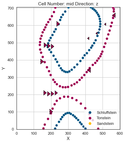
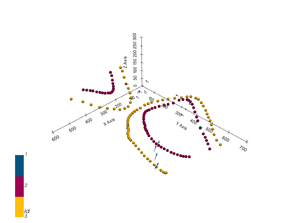
Plotting Input Data#
[34]:
gp.plot_2d(geo_model, direction='z', show_lith=False, show_boundaries=False)
plt.grid()
[35]:
gp.plot_3d(geo_model, image=False, plotter_type='basic', notebook=True)
[35]:
<gempy.plot.vista.GemPyToVista at 0x1e7ef0f5d30>
Setting the Interpolator#
[36]:
gp.set_interpolator(geo_model,
                    compile_theano=True,
                    theano_optimizer='fast_compile',
                    verbose=[],
                    update_kriging=False
                    )
Compiling theano function...
Level of Optimization:  fast_compile
Device:  cpu
Precision:  float64
Number of faults:  0
Compilation Done!
Kriging values:
                   values
range             973.77
$C_o$           22576.81
drift equations      [3]
[36]:
<gempy.core.interpolator.InterpolatorModel at 0x1e7e8161e50>
Computing Model#
[37]:
sol = gp.compute_model(geo_model, compute_mesh=True)
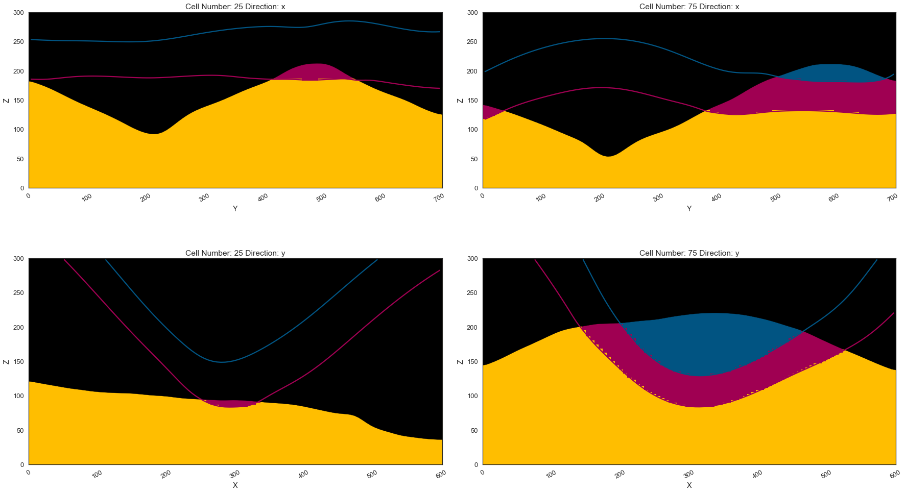
Plotting Cross Sections#
[38]:
fig = gp.plot_2d(geo_model, direction=['x', 'x', 'y', 'y'], cell_number=[25, 75, 25, 75], show_topography=True, show_data=False)
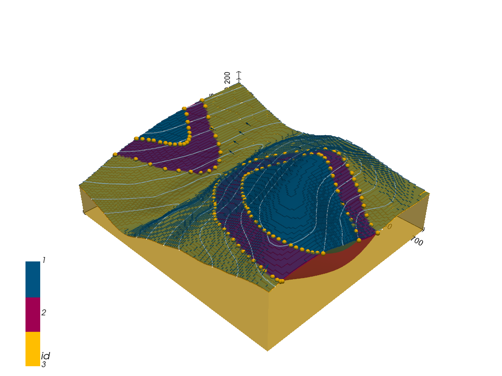
[39]:
gpv = gp.plot_3d(geo_model, image=False, show_topography=True,
                 plotter_type='basic', notebook=True, show_lith=True)
[ ]: