Example 25 - Planar Dipping Layers

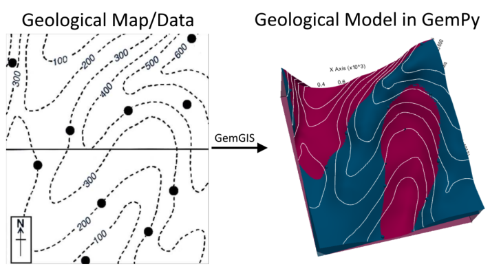
This example will show how to convert the geological map below using GemGIS to a GemPy model. This example is based on digitized data. The area is 1370 m wide (W-E extent) and 1561 m high (N-S extent). The model represents planar layers dipping towards the southwest.

The map has been georeferenced with QGIS. The stratigraphic boundaries were digitized in QGIS. Strikes lines were digitized in QGIS as well and will be used to calculate orientations for the GemPy model. The contour lines were also digitized and will be interpolated with GemGIS to create a topography for the model.

Map Source: Unknown

import matplotlib.pyplot as plt
import matplotlib.image as mpimg
img = mpimg.imread('../images/cover_example25.png')
plt.figure(figsize=(10, 10))
imgplot = plt.imshow(img)
plt.axis('off')
plt.tight_layout()

Licensing

Computational Geosciences and Reservoir Engineering, RWTH Aachen University, Authors: Alexander Juestel. For more information contact: alexander.juestel(at)rwth-aachen.de

This work is licensed under a Creative Commons Attribution 4.0 International License (http://creativecommons.org/licenses/by/4.0/)

Import GemGIS

If you have installed GemGIS via pip, you can import GemGIS like any other package. If you have downloaded the repository, append the path to the directory where the GemGIS repository is stored and then import GemGIS.

import warnings
warnings.filterwarnings("ignore")
import gemgis as gg

Importing Libraries and loading Data

All remaining packages can be loaded in order to prepare the data and to construct the model. The example data is downloaded form an external server using pooch. It will be stored in a data folder in the same directory where this notebook is stored.

import geopandas as gpd
import rasterio

file_path = 'data/example25/'
gg.download_gemgis_data.download_tutorial_data(filename="example25_planar_dipping_layers.zip", dirpath=file_path)

Downloading file 'example25_planar_dipping_layers.zip' from 'https://rwth-aachen.sciebo.de/s/AfXRsZywYDbUF34/download?path=%2Fexample25_planar_dipping_layers.zip' to 'C:\Users\ale93371\Documents\gemgis\docs\getting_started\data\example25'.

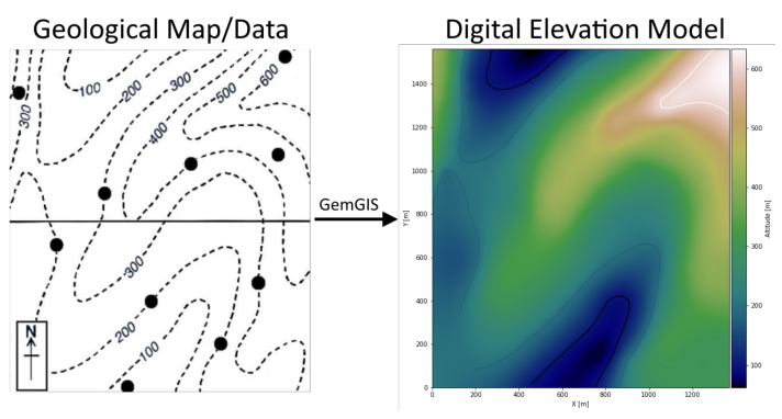
Creating Digital Elevation Model from Contour Lines

The digital elevation model (DEM) will be created by interpolating contour lines digitized from the georeferenced map using the SciPy Radial Basis Function interpolation wrapped in GemGIS. The respective function used for that is gg.vector.interpolate_raster().

img = mpimg.imread('../images/dem_example25.png')
plt.figure(figsize=(10, 10))
imgplot = plt.imshow(img)
plt.axis('off')
plt.tight_layout()

topo = gpd.read_file(file_path + 'topo25.shp')
topo.head()

	id	Z	geometry
0	None	100	LINESTRING (457.460 15.883, 503.059 59.552, 53...
1	None	200	LINESTRING (194.243 87.056, 230.432 90.433, 26...
2	None	200	LINESTRING (2.921 841.967, 15.225 879.122, 25....
3	None	400	LINESTRING (4.369 1340.899, 13.054 1365.026, 1...
4	None	300	LINESTRING (3.765 1021.105, 17.276 1062.120, 3...

Interpolating the contour lines

topo_raster = gg.vector.interpolate_raster(gdf=topo, value='Z', method='rbf', res=5)

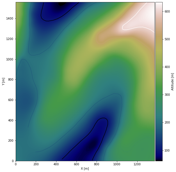
Plotting the raster

import matplotlib.pyplot as plt

from mpl_toolkits.axes_grid1 import make_axes_locatable

fix, ax = plt.subplots(1, figsize=(10,10))
topo.plot(ax=ax, aspect='equal', column='Z', cmap='gist_earth')
im = ax.imshow(topo_raster, origin='lower', extent=[0,1370,0,1561], cmap='gist_earth')
divider = make_axes_locatable(ax)
cax = divider.append_axes("right", size="5%", pad=0.05)
cbar = plt.colorbar(im, cax=cax)
cbar.set_label('Altitude [m]')
ax.set_xlabel('X [m]')
ax.set_ylabel('Y [m]')

Text(94.03793584379343, 0.5, 'Y [m]')

Saving the raster to disc

After the interpolation of the contour lines, the raster is saved to disc using gg.raster.save_as_tiff(). The function will not be executed as as raster is already provided with the example data.

gg.raster.save_as_tiff(raster=topo_raster, path=file_path + 'raster25.tif', extent=[0,1370,0,1561], crs='EPSG:4326', overwrite_file=True)

Opening Raster

The previously computed and saved raster can now be opened using rasterio.

topo_raster = rasterio.open(file_path + 'raster25.tif')

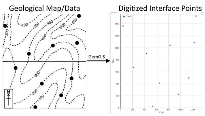
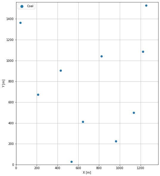
Interface Points of stratigraphic boundaries

The interface points will be extracted from LineStrings digitized from the georeferenced map using QGIS. It is important to provide a formation name for each layer boundary. The vertical position of the interface point will be extracted from the digital elevation model using the GemGIS function gg.vector.extract_xyz(). The resulting GeoDataFrame now contains single points including the information about the respective formation.

img = mpimg.imread('../images/interfaces_example25.png')
plt.figure(figsize=(10, 10))
imgplot = plt.imshow(img)
plt.axis('off')
plt.tight_layout()

interfaces = gpd.read_file(file_path + 'interfaces25.shp')
interfaces.head()

	id	formation	geometry
0	None	Coal	POINT (535.509 26.619)
1	None	Coal	POINT (963.992 223.490)
2	None	Coal	POINT (1135.771 497.565)
3	None	Coal	POINT (645.525 410.710)
4	None	Coal	POINT (213.182 671.274)

Extracting XY coordinates from Digital Elevation Model

interfaces_coords = gg.vector.extract_xyz(gdf=interfaces, dem=topo_raster)
interfaces_coords = interfaces_coords.sort_values(by='formation', ascending=False)
interfaces_coords.head()

	formation	geometry	X	Y	Z
0	Coal	POINT (535.509 26.619)	535.51	26.62	83.73
1	Coal	POINT (963.992 223.490)	963.99	223.49	198.26
2	Coal	POINT (1135.771 497.565)	1135.77	497.56	301.38
3	Coal	POINT (645.525 410.710)	645.52	410.71	199.98
4	Coal	POINT (213.182 671.274)	213.18	671.27	199.13

Plotting the Interface Points

fig, ax = plt.subplots(1, figsize=(10,10))

interfaces.plot(ax=ax, column='formation', legend=True, aspect='equal')
interfaces_coords.plot(ax=ax, column='formation', legend=True, aspect='equal')
plt.grid()
plt.xlabel('X [m]')
plt.ylabel('Y [m]')
plt.xlim(0,1370)
plt.ylim(0,1561)

(0.0, 1561.0)

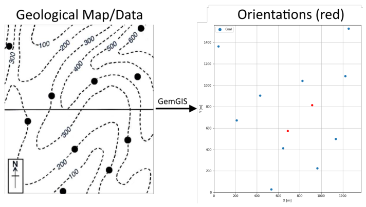
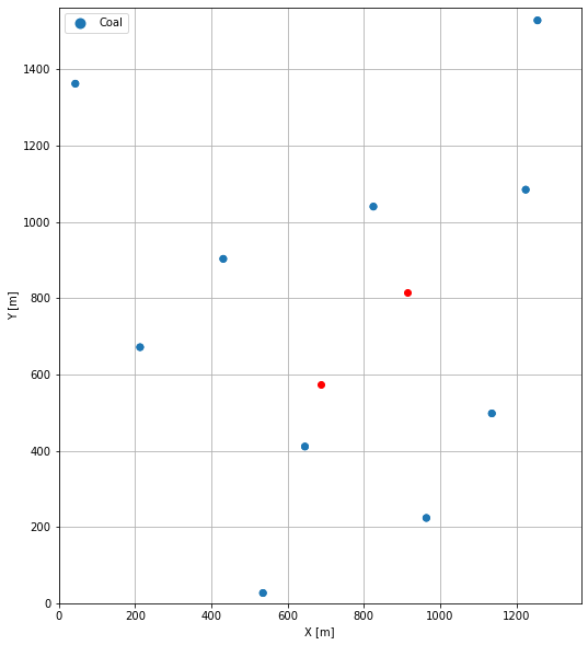
Orientations from Strike Lines

Strike lines connect outcropping stratigraphic boundaries (interfaces) of the same altitude. In other words: the intersections between topographic contours and stratigraphic boundaries at the surface. The height difference and the horizontal difference between two digitized lines is used to calculate the dip and azimuth and hence an orientation that is necessary for GemPy. In order to calculate the orientations, each set of strikes lines/LineStrings for one formation must be given an id number next to the altitude of the strike line. The id field is already predefined in QGIS. The strike line with the lowest altitude gets the id number 1, the strike line with the highest altitude the the number according to the number of digitized strike lines. It is currently recommended to use one set of strike lines for each structural element of one formation as illustrated.

img = mpimg.imread('../images/orientations_example25.png')
plt.figure(figsize=(10, 10))
imgplot = plt.imshow(img)
plt.axis('off')
plt.tight_layout()

strikes = gpd.read_file(file_path + 'strikes25.shp')
strikes

	id	formation	Z	geometry
0	1	Coal	200	LINESTRING (214.147 670.791, 968.817 221.077)
1	2	Coal	300	LINESTRING (432.248 905.299, 1137.701 501.907)
2	3	Coal	400	LINESTRING (828.885 1042.336, 1251.577 804.934)

Calculate Orientations for each formation

orientations_coal = gg.vector.calculate_orientations_from_strike_lines(gdf=strikes[strikes['formation']=='Coal'].sort_values(by='Z', ascending=True).reset_index())
orientations_coal

	dip	azimuth	Z	geometry	polarity	formation	X	Y
0	17.71	210.32	250.00	POINT (688.228 574.769)	1.00	Coal	688.23	574.77
1	17.57	209.65	350.00	POINT (912.603 813.619)	1.00	Coal	912.60	813.62

Merging Orientations

import pandas as pd
orientations = pd.concat([orientations_coal]).reset_index()
orientations['formation'] = 'Coal'
orientations

	index	dip	azimuth	Z	geometry	polarity	formation	X	Y
0	0	17.71	210.32	250.00	POINT (688.228 574.769)	1.00	Coal	688.23	574.77
1	1	17.57	209.65	350.00	POINT (912.603 813.619)	1.00	Coal	912.60	813.62

Plotting the Orientations

fig, ax = plt.subplots(1, figsize=(10,10))

interfaces.plot(ax=ax, column='formation', legend=True, aspect='equal')
interfaces_coords.plot(ax=ax, column='formation', legend=True, aspect='equal')
orientations.plot(ax=ax, color='red', aspect='equal')
plt.grid()
plt.xlabel('X [m]')
plt.ylabel('Y [m]')
plt.xlim(0,1370)
plt.ylim(0,1561)

(0.0, 1561.0)

GemPy Model Construction

The structural geological model will be constructed using the GemPy package.

import gempy as gp

WARNING (theano.configdefaults): g++ not available, if using conda: `conda install m2w64-toolchain`
WARNING (theano.configdefaults): g++ not detected ! Theano will be unable to execute optimized C-implementations (for both CPU and GPU) and will default to Python implementations. Performance will be severely degraded. To remove this warning, set Theano flags cxx to an empty string.
WARNING (theano.tensor.blas): Using NumPy C-API based implementation for BLAS functions.

Creating new Model

geo_model = gp.create_model('Model25')
geo_model

Model25  2022-04-09 09:01

Initiate Data

gp.init_data(geo_model, [0,1370,0,1561,0,800], [100,100,100],
             surface_points_df = interfaces_coords[interfaces_coords['Z']!=0],
             orientations_df = orientations,
             default_values=True)

Active grids: ['regular']

Model25  2022-04-09 09:01

Model Surfaces

geo_model.surfaces

	surface	series	order_surfaces	color	id
0	Coal	Default series	1	#015482	1

Mapping the Stack to Surfaces

gp.map_stack_to_surfaces(geo_model,
                         {
                          'Strata1': ('Coal'),
                         },
                         remove_unused_series=True)
geo_model.add_surfaces('Basement')

	surface	series	order_surfaces	color	id
0	Coal	Strata1	1	#015482	1
1	Basement	Strata1	2	#9f0052	2

Showing the Number of Data Points

gg.utils.show_number_of_data_points(geo_model=geo_model)

	surface	series	order_surfaces	color	id	No. of Interfaces	No. of Orientations
0	Coal	Strata1	1	#015482	1	10	2
1	Basement	Strata1	2	#9f0052	2	0	0

Loading Digital Elevation Model

geo_model.set_topography(
    source='gdal', filepath=file_path + 'raster25.tif')

Cropped raster to geo_model.grid.extent.
depending on the size of the raster, this can take a while...
storing converted file...
Active grids: ['regular' 'topography']

Grid Object. Values:
array([[   6.85      ,    7.805     ,    4.        ],
       [   6.85      ,    7.805     ,   12.        ],
       [   6.85      ,    7.805     ,   20.        ],
       ...,
       [1367.5       , 1548.49198718,  622.15332031],
       [1367.5       , 1553.49519231,  620.90863037],
       [1367.5       , 1558.49839744,  619.59674072]])

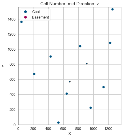
Plotting Input Data

gp.plot_2d(geo_model, direction='z', show_lith=False, show_boundaries=False)
plt.grid()

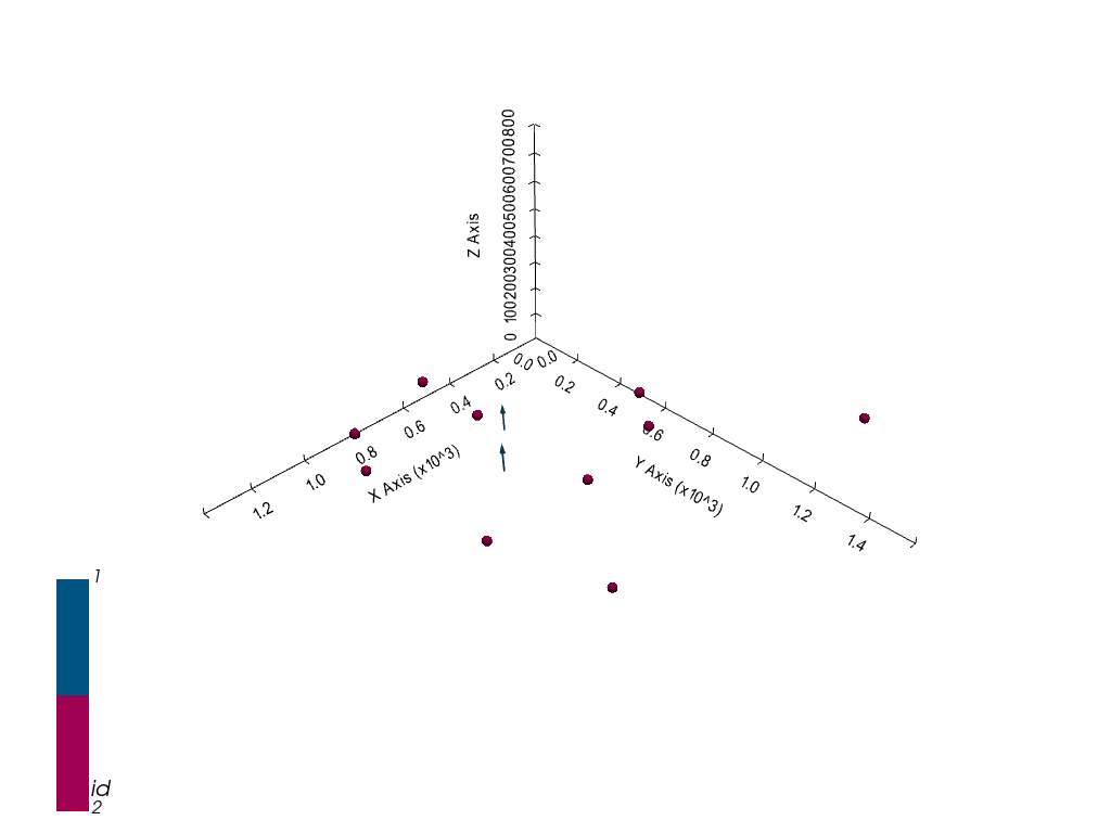
gp.plot_3d(geo_model, image=False, plotter_type='basic', notebook=True)

<gempy.plot.vista.GemPyToVista at 0x2582e21b460>

Setting the Interpolator

gp.set_interpolator(geo_model,
                    compile_theano=True,
                    theano_optimizer='fast_compile',
                    verbose=[],
                    update_kriging = False
                    )

Compiling theano function...
Level of Optimization:  fast_compile
Device:  cpu
Precision:  float64
Number of faults:  0
Compilation Done!
Kriging values:
                    values
range             2225.67
$C_o$           117943.36
drift equations       [3]

<gempy.core.interpolator.InterpolatorModel at 0x258274bbdc0>

Computing Model

sol = gp.compute_model(geo_model, compute_mesh=True)

Plotting Cross Sections

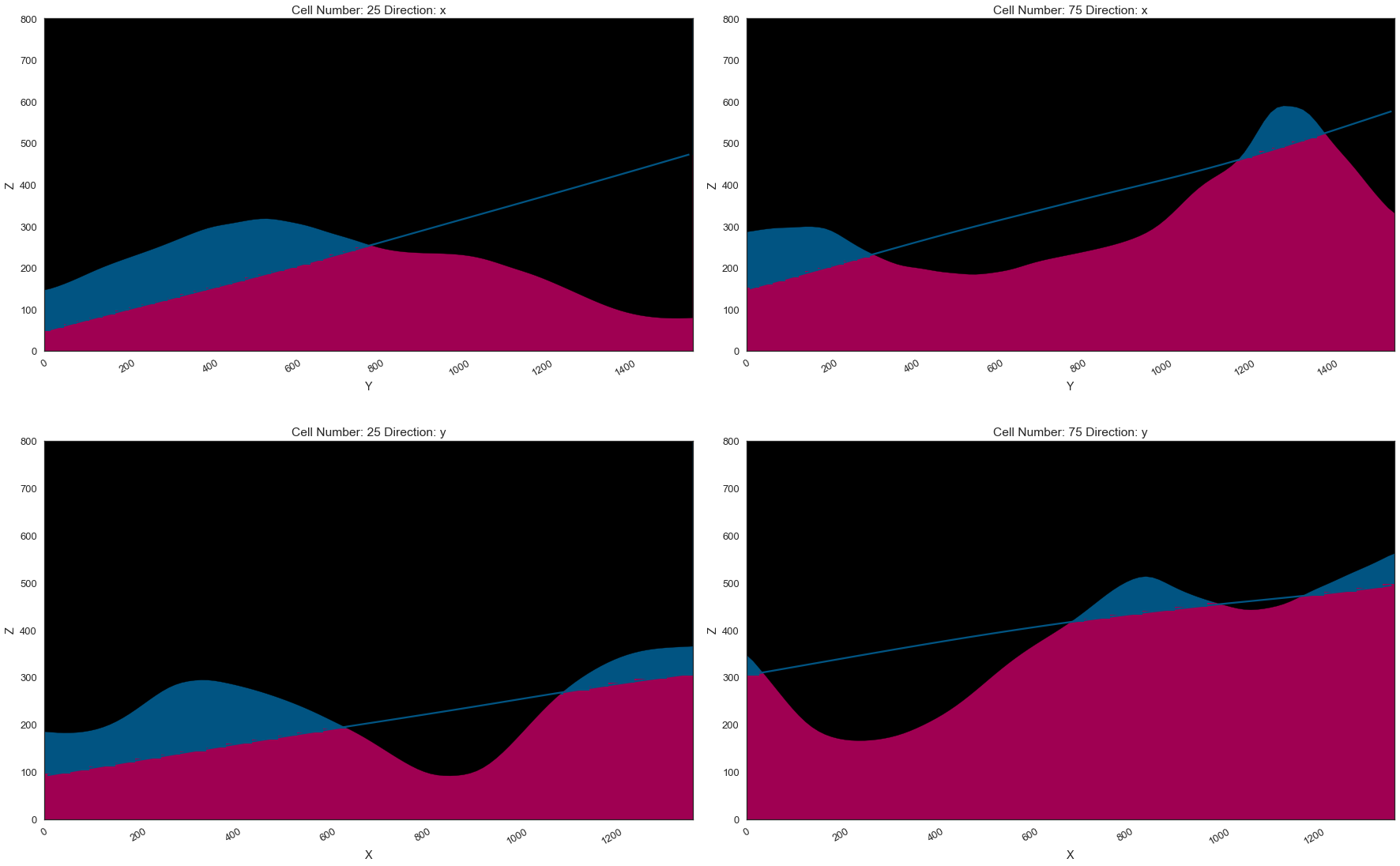
gp.plot_2d(geo_model, direction=['x', 'x', 'y', 'y'], cell_number=[25,75,25,75], show_topography=True, show_data=False)

<gempy.plot.visualization_2d.Plot2D at 0x25834904490>

Plotting 3D Model

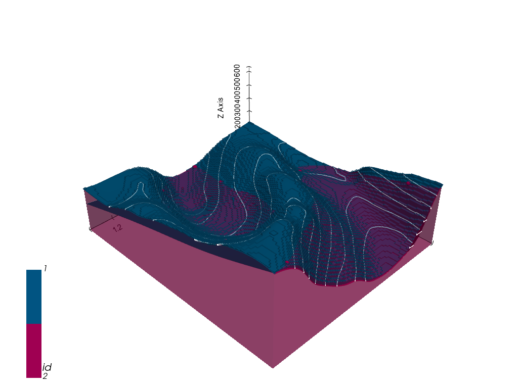
gpv = gp.plot_3d(geo_model, image=False, show_topography=True,
                 plotter_type='basic', notebook=True, show_lith=True)