
Example 10 - Faulted Folded Layers
Contents
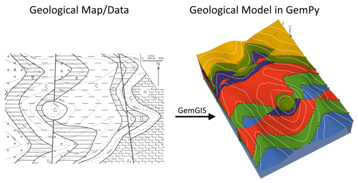
Example 10 - Faulted Folded Layers#
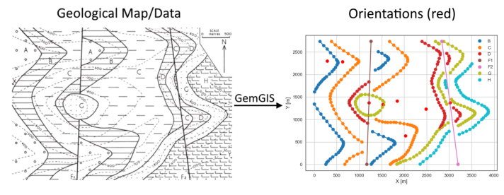
This example will show how to convert the geological map below using GemGIS to a GemPy model. This example is based on digitized data. The area is 3954 m wide (W-E extent) and 2738 m high (N-S extent). The vertical model extent varies between 0 m and 1000 m. The model represents folded layers (yellow to light green) which are separated to a second set of layers (blue and purple) by an unconformity. A light blue layer represents the basement. The map has been georeferenced with QGIS. The
stratigraphic boundaries were digitized in QGIS. Strikes lines were digitized in QGIS as well and will be used to calculate orientations for the GemPy model. The contour lines were also digitized and will be interpolated with GemGIS to create a topography for the model.
Map Source: An Introduction to Geological Structures and Maps by G.M. Bennison
[1]:
import matplotlib.pyplot as plt
import matplotlib.image as mpimg
img = mpimg.imread('../images/cover_example10.png')
plt.figure(figsize=(10, 10))
imgplot = plt.imshow(img)
plt.axis('off')
plt.tight_layout()
Licensing#
Computational Geosciences and Reservoir Engineering, RWTH Aachen University, Authors: Alexander Juestel. For more information contact: alexander.juestel(at)rwth-aachen.de
This work is licensed under a Creative Commons Attribution 4.0 International License (http://creativecommons.org/licenses/by/4.0/)
Import GemGIS#
If you have installed GemGIS via pip or conda, you can import GemGIS like any other package. If you have downloaded the repository, append the path to the directory where the GemGIS repository is stored and then import GemGIS.
[2]:
import warnings
warnings.filterwarnings("ignore")
import gemgis as gg
Importing Libraries and loading Data#
All remaining packages can be loaded in order to prepare the data and to construct the model. The example data is downloaded from an external server using pooch. It will be stored in a data folder in the same directory where this notebook is stored.
[3]:
import geopandas as gpd
import rasterio
[4]:
file_path = 'data/example10/'
gg.download_gemgis_data.download_tutorial_data(filename="example10_faulted_folded_layers.zip", dirpath=file_path)
Downloading file 'example10_faulted_folded_layers.zip' from 'https://rwth-aachen.sciebo.de/s/AfXRsZywYDbUF34/download?path=%2Fexample10_faulted_folded_layers.zip' to 'C:\Users\ale93371\Documents\gemgis\docs\getting_started\example\data\example10'.
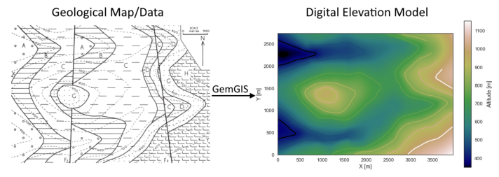
Creating Digital Elevation Model from Contour Lines#
The digital elevation model (DEM) will be created by interpolating contour lines digitized from the georeferenced map using the SciPy Radial Basis Function interpolation wrapped in GemGIS. The respective function used for that is gg.vector.interpolate_raster().
[5]:
import matplotlib.pyplot as plt
import matplotlib.image as mpimg
img = mpimg.imread('../images/dem_example10.png')
plt.figure(figsize=(10, 10))
imgplot = plt.imshow(img)
plt.axis('off')
plt.tight_layout()
[6]:
topo = gpd.read_file(file_path + 'topo10.shp')
topo.head()
[6]:
| id | Z | geometry | |
|---|---|---|---|
| 0 | None | 600 | LINESTRING (500.103 2733.663, 594.070 2684.564... |
| 1 | None | 500 | LINESTRING (217.356 2726.044, 324.445 2643.506... |
| 2 | None | 400 | LINESTRING (11.222 2589.327, 69.634 2556.312, ... |
| 3 | None | 900 | LINESTRING (1037.237 1522.677, 1083.798 1526.9... |
| 4 | None | 800 | LINESTRING (912.795 1610.718, 990.677 1620.030... |
Interpolating the contour lines#
[7]:
topo_raster = gg.vector.interpolate_raster(gdf=topo, value='Z', method='rbf', res=10)
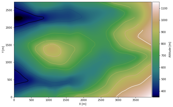
Plotting the raster#
[8]:
import matplotlib.pyplot as plt
from mpl_toolkits.axes_grid1 import make_axes_locatable

fix, ax = plt.subplots(1, figsize=(10, 10))
topo.plot(ax=ax, aspect='equal', column='Z', cmap='gist_earth')
im = plt.imshow(topo_raster, origin='lower', extent=[0, 3954, 0, 2738], cmap='gist_earth')
divider = make_axes_locatable(ax)
cax = divider.append_axes("right", size="5%", pad=0.05)
cbar = plt.colorbar(im, cax=cax)
cbar.set_label('Altitude [m]')
ax.set_xlabel('X [m]')
ax.set_ylabel('Y [m]')
ax.set_xlim(0, 3954)
ax.set_ylim(0, 2738)
[8]:
(0.0, 2738.0)
Saving the raster to disc#
After the interpolation of the contour lines, the raster is saved to disc using gg.raster.save_as_tiff(). The function will not be executed as a raster is already provided with the example data.
Opening Raster#
The previously computed and saved raster can now be opened using rasterio.
[9]:
topo_raster = rasterio.open(file_path + 'raster10.tif')
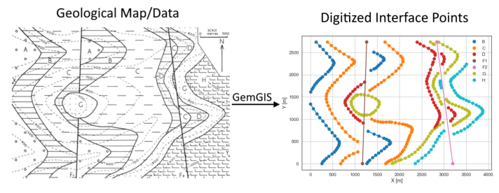
Interface Points of stratigraphic boundaries#
The interface points will be extracted from LineStrings digitized from the georeferenced map using QGIS. It is important to provide a formation name for each layer boundary. The vertical position of the interface point will be extracted from the digital elevation model using the GemGIS function gg.vector.extract_xyz(). The resulting GeoDataFrame now contains single points including the information about the respective formation.
[10]:
import matplotlib.pyplot as plt
import matplotlib.image as mpimg
img = mpimg.imread('../images/interfaces_example10.png')
plt.figure(figsize=(10, 10))
imgplot = plt.imshow(img)
plt.axis('off')
plt.tight_layout()
[11]:
interfaces = gpd.read_file(file_path + 'interfaces10.shp')
interfaces.head()
[11]:
| id | formation | geometry | |
|---|---|---|---|
| 0 | None | F1 | LINESTRING (1263.266 2736.203, 1170.145 1.855) |
| 1 | None | F2 | LINESTRING (2839.537 2736.203, 3198.049 1.855) |
| 2 | None | B | LINESTRING (128.046 2733.240, 211.007 2641.813... |
| 3 | None | B | LINESTRING (3.603 1339.823, 67.941 1234.851, 1... |
| 4 | None | C | LINESTRING (681.688 2.279, 724.862 66.616, 789... |
Extracting Z coordinate from Digital Elevation Model#
[12]:
interfaces_coords = gg.vector.extract_xyz(gdf=interfaces, dem=topo_raster)
interfaces_coords = interfaces_coords.sort_values(by='formation', ascending=False)
interfaces_coords.head()
[12]:
| formation | geometry | X | Y | Z | |
|---|---|---|---|---|---|
| 322 | H | POINT (2940.276 1706.378) | 2940.28 | 1706.38 | 814.55 |
| 371 | H | POINT (3262.810 1592.094) | 3262.81 | 1592.09 | 879.04 |
| 369 | H | POINT (3188.314 1716.537) | 3188.31 | 1716.54 | 888.36 |
| 368 | H | POINT (3162.071 1769.023) | 3162.07 | 1769.02 | 887.87 |
| 367 | H | POINT (3148.526 1840.979) | 3148.53 | 1840.98 | 889.10 |
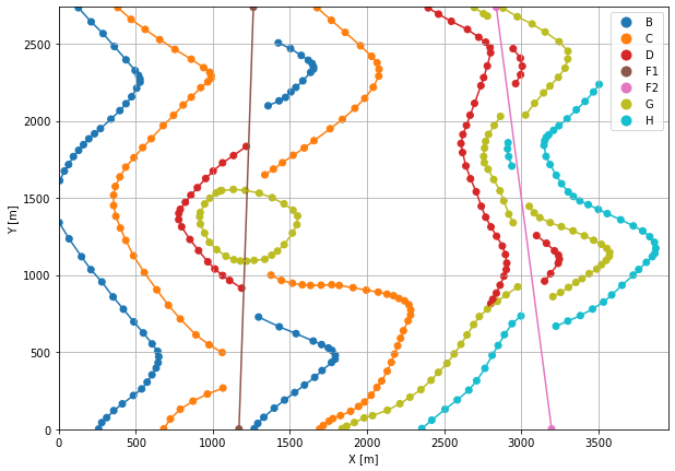
Plotting the Interface Points#
[13]:
fig, ax = plt.subplots(1, figsize=(10, 10))

interfaces.plot(ax=ax, column='formation', legend=True, aspect='equal')
interfaces_coords.plot(ax=ax, column='formation', legend=True, aspect='equal')
plt.grid()
ax.set_xlabel('X [m]')
ax.set_ylabel('Y [m]')
ax.set_xlim(0, 3954)
ax.set_ylim(0, 2738)
[13]:
(0.0, 2738.0)
Orientations from Strike Lines#
Strike lines connect outcropping stratigraphic boundaries (interfaces) of the same altitude. In other words: the intersections between topographic contours and stratigraphic boundaries at the surface. The height difference and the horizontal difference between two digitized lines is used to calculate the dip and azimuth and hence an orientation that is necessary for GemPy. In order to calculate the orientations, each set of strikes lines/LineStrings for one formation must be given an id
number next to the altitude of the strike line. The id field is already predefined in QGIS. The strike line with the lowest altitude gets the id number 1, the strike line with the highest altitude the the number according to the number of digitized strike lines. It is currently recommended to use one set of strike lines for each structural element of one formation as illustrated.
[14]:
import matplotlib.pyplot as plt
import matplotlib.image as mpimg
img = mpimg.imread('../images/orientations_example10.png')
plt.figure(figsize=(10, 10))
imgplot = plt.imshow(img)
plt.axis('off')
plt.tight_layout()
[15]:
strikes = gpd.read_file(file_path + 'strikes10.shp')
strikes.head()
[15]:
| id | formation | Z | geometry | |
|---|---|---|---|---|
| 0 | 1.00 | B | 400 | LINESTRING (416.718 2417.478, 467.511 2152.509) |
| 1 | 2.00 | B | 500 | LINESTRING (216.087 1913.782, 39.158 2721.388) |
| 2 | NaN | B1 | 500 | LINESTRING (505.606 676.130, 576.716 313.808) |
| 3 | 1.00 | C | 500 | LINESTRING (751.105 2464.038, 832.373 2115.261) |
| 4 | 2.00 | C | 600 | LINESTRING (549.626 1825.741, 375.238 2734.933) |
Calculate Orientations for each formation#
[16]:
orientations_f1 = gg.vector.calculate_orientations_from_strike_lines(gdf=strikes[strikes['formation'] == 'F1'].sort_values(by='Z', ascending=True).reset_index())
orientations_f1
[16]:
| dip | azimuth | Z | geometry | polarity | formation | X | Y | |
|---|---|---|---|---|---|---|---|---|
| 0 | 89.75 | 91.97 | 1000.00 | POINT (1216.176 1369.029) | 1.00 | F1 | 1216.18 | 1369.03 |
[17]:
orientations_f2 = gg.vector.calculate_orientations_from_strike_lines(gdf=strikes[strikes['formation'] == 'F2'].sort_values(by='Z', ascending=True).reset_index())
orientations_f2
[17]:
| dip | azimuth | Z | geometry | polarity | formation | X | Y | |
|---|---|---|---|---|---|---|---|---|
| 0 | 89.75 | 82.52 | 1000.00 | POINT (3018.793 1368.818) | 1.00 | F2 | 3018.79 | 1368.82 |
[18]:
orientations_c2 = gg.vector.calculate_orientations_from_strike_lines(gdf=strikes[strikes['formation'] == 'C2'].sort_values(by='Z', ascending=True).reset_index())
orientations_c2
[18]:
| dip | azimuth | Z | geometry | polarity | formation | X | Y | |
|---|---|---|---|---|---|---|---|---|
| 0 | 16.56 | 76.45 | 650.00 | POINT (1845.267 1413.896) | 1.00 | C2 | 1845.27 | 1413.90 |
| 1 | 17.33 | 76.32 | 750.00 | POINT (1524.849 1332.628) | 1.00 | C2 | 1524.85 | 1332.63 |
[19]:
orientations_c = gg.vector.calculate_orientations_from_strike_lines(gdf=strikes[strikes['formation'] == 'C'].sort_values(by='Z', ascending=True).reset_index())
orientations_c
[19]:
| dip | azimuth | Z | geometry | polarity | formation | X | Y | |
|---|---|---|---|---|---|---|---|---|
| 0 | 17.45 | 78.85 | 550.00 | POINT (627.085 2284.993) | 1.00 | C | 627.09 | 2284.99 |
[20]:
orientations_c1 = gg.vector.calculate_orientations_from_strike_lines(gdf=strikes[strikes['formation'] == 'C1'].sort_values(by='Z', ascending=True).reset_index())
orientations_c1
[20]:
| dip | azimuth | Z | geometry | polarity | formation | X | Y | |
|---|---|---|---|---|---|---|---|---|
| 0 | 16.85 | 76.63 | 650.00 | POINT (2029.391 637.612) | 1.00 | C1 | 2029.39 | 637.61 |
[21]:
orientations_b = gg.vector.calculate_orientations_from_strike_lines(gdf=strikes[strikes['formation'] == 'B'].sort_values(by='Z', ascending=True).reset_index())
orientations_b
[21]:
| dip | azimuth | Z | geometry | polarity | formation | X | Y | |
|---|---|---|---|---|---|---|---|---|
| 0 | 18.63 | 77.79 | 450.00 | POINT (284.869 2301.289) | 1.00 | B | 284.87 | 2301.29 |
[22]:
orientations_g = gg.vector.calculate_orientations_from_strike_lines(gdf=strikes[strikes['formation'] == 'G'].sort_values(by='Z', ascending=True).reset_index())
orientations_g
[22]:
| dip | azimuth | Z | geometry | polarity | formation | X | Y | |
|---|---|---|---|---|---|---|---|---|
| 0 | 6.00 | 90.92 | 750.00 | POINT (2481.976 1233.264) | 1.00 | G | 2481.98 | 1233.26 |
Merging Orientations#
[23]:
import pandas as pd
orientations = pd.concat([orientations_f1, orientations_f2, orientations_c2, orientations_c, orientations_c1, orientations_b, orientations_g]).reset_index()
orientations['formation'] = ['F1', 'F2', 'C', 'C', 'C', 'C', 'B', 'G']
orientations = orientations[orientations['formation'].isin(['F1', 'F2', 'C', 'B', 'G'])]
orientations
[23]:
| index | dip | azimuth | Z | geometry | polarity | formation | X | Y | |
|---|---|---|---|---|---|---|---|---|---|
| 0 | 0 | 89.75 | 91.97 | 1000.00 | POINT (1216.176 1369.029) | 1.00 | F1 | 1216.18 | 1369.03 |
| 1 | 0 | 89.75 | 82.52 | 1000.00 | POINT (3018.793 1368.818) | 1.00 | F2 | 3018.79 | 1368.82 |
| 2 | 0 | 16.56 | 76.45 | 650.00 | POINT (1845.267 1413.896) | 1.00 | C | 1845.27 | 1413.90 |
| 3 | 1 | 17.33 | 76.32 | 750.00 | POINT (1524.849 1332.628) | 1.00 | C | 1524.85 | 1332.63 |
| 4 | 0 | 17.45 | 78.85 | 550.00 | POINT (627.085 2284.993) | 1.00 | C | 627.09 | 2284.99 |
| 5 | 0 | 16.85 | 76.63 | 650.00 | POINT (2029.391 637.612) | 1.00 | C | 2029.39 | 637.61 |
| 6 | 0 | 18.63 | 77.79 | 450.00 | POINT (284.869 2301.289) | 1.00 | B | 284.87 | 2301.29 |
| 7 | 0 | 6.00 | 90.92 | 750.00 | POINT (2481.976 1233.264) | 1.00 | G | 2481.98 | 1233.26 |
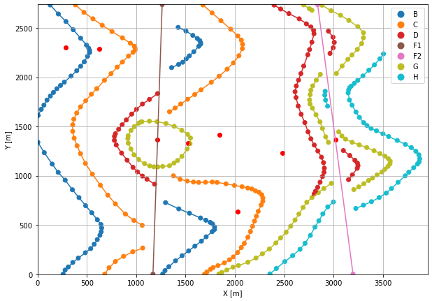
Plotting the Orientations#
[24]:
fig, ax = plt.subplots(1, figsize=(10, 10))

interfaces.plot(ax=ax, column='formation', legend=True, aspect='equal')
interfaces_coords.plot(ax=ax, column='formation', legend=True, aspect='equal')
orientations.plot(ax=ax, color='red', aspect='equal')
plt.grid()
ax.set_xlabel('X [m]')
ax.set_ylabel('Y [m]')
ax.set_xlim(0, 3954)
ax.set_ylim(0, 2738)
[24]:
(0.0, 2738.0)
GemPy Model Construction#
The structural geological model will be constructed using the GemPy package.
[25]:
import gempy as gp
WARNING (theano.configdefaults): g++ not available, if using conda: `conda install m2w64-toolchain`
WARNING (theano.configdefaults): g++ not detected ! Theano will be unable to execute optimized C-implementations (for both CPU and GPU) and will default to Python implementations. Performance will be severely degraded. To remove this warning, set Theano flags cxx to an empty string.
WARNING (theano.tensor.blas): Using NumPy C-API based implementation for BLAS functions.
Creating new Model#
[26]:
geo_model = gp.create_model('Model10')
geo_model
[26]:
Model10 2022-04-05 10:47
Initiate Data#
[27]:
gp.init_data(geo_model, [0, 3954, 0, 2738, 0, 1000], [100, 100, 100],
             surface_points_df=interfaces_coords[interfaces_coords['Z'] != 0],
             orientations_df=orientations,
             default_values=True)
Active grids: ['regular']
[27]:
Model10 2022-04-05 10:47
Model Surfaces#
[28]:
geo_model.surfaces
[28]:
| surface | series | order_surfaces | color | id | |
|---|---|---|---|---|---|
| 0 | H | Default series | 1 | #015482 | 1 |
| 1 | G | Default series | 2 | #9f0052 | 2 |
| 2 | F2 | Default series | 3 | #ffbe00 | 3 |
| 3 | F1 | Default series | 4 | #728f02 | 4 |
| 4 | D | Default series | 5 | #443988 | 5 |
| 5 | C | Default series | 6 | #ff3f20 | 6 |
| 6 | B | Default series | 7 | #5DA629 | 7 |
Mapping the Stack to Surfaces#
[29]:
gp.map_stack_to_surfaces(geo_model,
                         {
                          'Fault1': ('F1'),
                          'Fault2': ('F2'),
                          'Strata1': ('H', 'G'),
                          'Strata2': ('D', 'C', 'B'),
                         },
                         remove_unused_series=True)
geo_model.add_surfaces('Basement')
geo_model.set_is_fault(['Fault1', 'Fault2'])
Fault colors changed. If you do not like this behavior, set change_color to False.
[29]:
| order_series | BottomRelation | isActive | isFault | isFinite | |
|---|---|---|---|---|---|
| Fault1 | 1 | Fault | True | True | False |
| Fault2 | 2 | Fault | True | True | False |
| Strata1 | 3 | Erosion | True | False | False |
| Strata2 | 4 | Erosion | True | False | False |
Adding additional Orientations#
[30]:
geo_model.add_orientations(X=1200, Y=1350, Z=1025, surface='G', orientation=[90,5,1])
geo_model.add_orientations(X=3500, Y=350, Z=1000, surface='G', orientation=[90,6,1])
geo_model.add_orientations(X=3500, Y=350, Z=1000, surface='H', orientation=[90,6,1])
geo_model.add_orientations(X=3500, Y=2000, Z=1000, surface='G', orientation=[90,6,1])
geo_model.add_orientations(X=3500, Y=2000, Z=1000, surface='H', orientation=[90,6,1])
geo_model.add_orientations(X=2800, Y=2000, Z=1000, surface='D', orientation=[90,18,1])
geo_model.add_orientations(X=2800, Y=1000, Z=1000, surface='D', orientation=[90,18,1])
[30]:
| X | Y | Z | G_x | G_y | G_z | smooth | surface | |
|---|---|---|---|---|---|---|---|---|
| 0 | 1216.18 | 1369.03 | 1000.00 | 1.00 | -0.03 | 0.00 | 0.01 | F1 |
| 1 | 3018.79 | 1368.82 | 1000.00 | 0.99 | 0.13 | 0.00 | 0.01 | F2 |
| 10 | 3500.00 | 350.00 | 1000.00 | 0.10 | 0.00 | 0.99 | 0.01 | H |
| 12 | 3500.00 | 2000.00 | 1000.00 | 0.10 | 0.00 | 0.99 | 0.01 | H |
| 7 | 2481.98 | 1233.26 | 750.00 | 0.10 | -0.00 | 0.99 | 0.01 | G |
| 8 | 1200.00 | 1350.00 | 1025.00 | 0.09 | 0.00 | 1.00 | 0.01 | G |
| 9 | 3500.00 | 350.00 | 1000.00 | 0.10 | 0.00 | 0.99 | 0.01 | G |
| 11 | 3500.00 | 2000.00 | 1000.00 | 0.10 | 0.00 | 0.99 | 0.01 | G |
| 13 | 2800.00 | 2000.00 | 1000.00 | 0.31 | 0.00 | 0.95 | 0.01 | D |
| 14 | 2800.00 | 1000.00 | 1000.00 | 0.31 | 0.00 | 0.95 | 0.01 | D |
| 2 | 1845.27 | 1413.90 | 650.00 | 0.28 | 0.07 | 0.96 | 0.01 | C |
| 3 | 1524.85 | 1332.63 | 750.00 | 0.29 | 0.07 | 0.95 | 0.01 | C |
| 4 | 627.09 | 2284.99 | 550.00 | 0.29 | 0.06 | 0.95 | 0.01 | C |
| 5 | 2029.39 | 637.61 | 650.00 | 0.28 | 0.07 | 0.96 | 0.01 | C |
| 6 | 284.87 | 2301.29 | 450.00 | 0.31 | 0.07 | 0.95 | 0.01 | B |
Showing the Number of Data Points#
[31]:
gg.utils.show_number_of_data_points(geo_model=geo_model)
[31]:
| surface | series | order_surfaces | color | id | No. of Interfaces | No. of Orientations | |
|---|---|---|---|---|---|---|---|
| 3 | F1 | Fault1 | 1 | #527682 | 1 | 2 | 1 |
| 2 | F2 | Fault2 | 1 | #527682 | 2 | 2 | 1 |
| 0 | H | Strata1 | 1 | #ffbe00 | 3 | 55 | 2 |
| 1 | G | Strata1 | 2 | #728f02 | 4 | 100 | 4 |
| 4 | D | Strata2 | 1 | #443988 | 5 | 65 | 2 |
| 5 | C | Strata2 | 2 | #ff3f20 | 6 | 96 | 4 |
| 6 | B | Strata2 | 3 | #5DA629 | 7 | 79 | 1 |
| 7 | Basement | Strata2 | 4 | #4878d0 | 8 | 0 | 0 |
Loading Digital Elevation Model#
[32]:
geo_model.set_topography(
    source='gdal', filepath=file_path + 'raster10.tif')
Cropped raster to geo_model.grid.extent.
depending on the size of the raster, this can take a while...
storing converted file...
Active grids: ['regular' 'topography']
[32]:
Grid Object. Values:
array([[  19.77      ,   13.69      ,    5.        ],
       [  19.77      ,   13.69      ,   15.        ],
       [  19.77      ,   13.69      ,   25.        ],
       ...,
       [3948.99493671, 2713.01824818, 1023.34295654],
       [3948.99493671, 2723.01094891, 1024.94226074],
       [3948.99493671, 2733.00364964, 1026.57104492]])
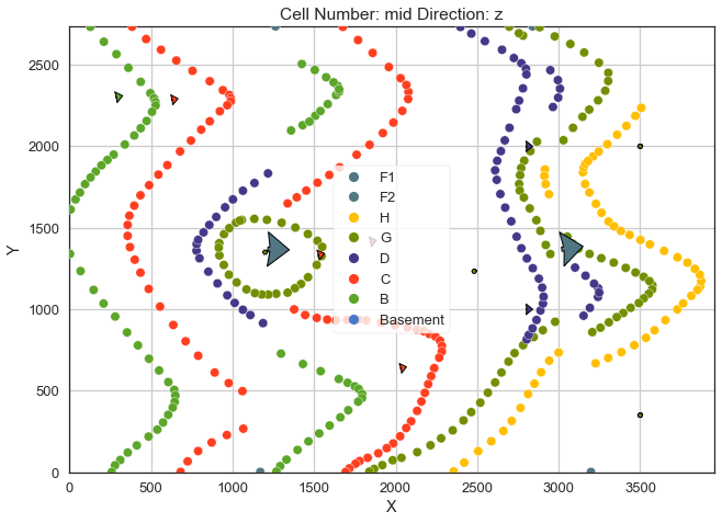
Plotting Input Data#
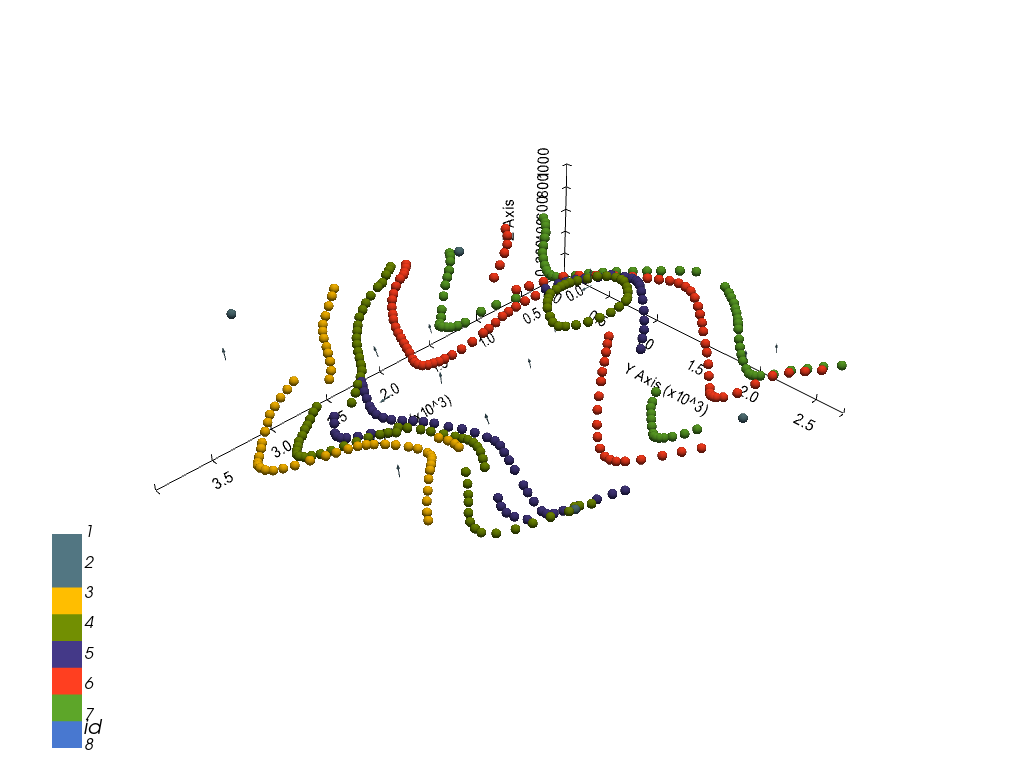
[33]:
gp.plot_2d(geo_model, direction='z', show_lith=False, show_boundaries=False)
plt.grid()
[34]:
gp.plot_3d(geo_model, image=False, plotter_type='basic', notebook=True)
[34]:
<gempy.plot.vista.GemPyToVista at 0x1da0740ba90>
Setting the Interpolator#
[35]:
gp.set_interpolator(geo_model,
                    compile_theano=True,
                    theano_optimizer='fast_compile',
                    verbose=[],
                    update_kriging=False
                    )
Compiling theano function...
Level of Optimization:  fast_compile
Device:  cpu
Precision:  float64
Number of faults:  2
Compilation Done!
Kriging values:
                        values
range                 4912.31
$C_o$                574541.9
drift equations  [3, 3, 3, 3]
[35]:
<gempy.core.interpolator.InterpolatorModel at 0x1da06704df0>
Computing Model#
[36]:
sol = gp.compute_model(geo_model, compute_mesh=True)
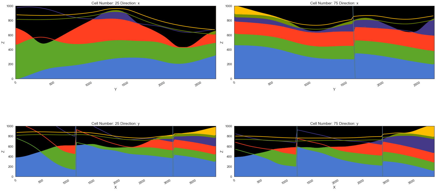
Plotting Cross Sections#
[37]:
gp.plot_2d(geo_model, direction=['x', 'x', 'y', 'y'], cell_number=[25, 75, 25, 75], show_topography=True, show_data=False)
[37]:
<gempy.plot.visualization_2d.Plot2D at 0x1da09edd640>
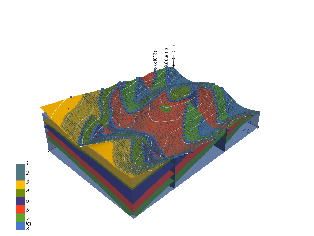
Plotting 3D Model#
[38]:
gpv = gp.plot_3d(geo_model, image=False, show_topography=True,
                 plotter_type='basic', notebook=True, show_lith=True)
[ ]: