
Example 18 - Faulted Folded Layers
Contents
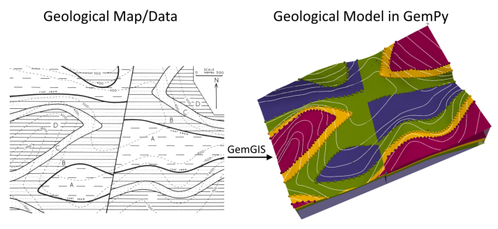
Example 18 - Faulted Folded Layers#
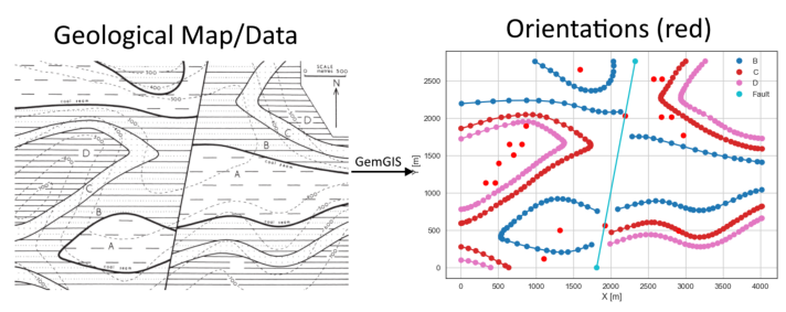
This example will show how to convert the geological map below using GemGIS to a GemPy model. This example is based on digitized data. The area is 4022 m wide (W-E extent) and 2761 m high (N-S extent). The vertical model extent varies between 0 m and 1000 m. The model represents folded layers which are cut by a roughly N-S trending fault.
The map has been georeferenced with QGIS. The stratigraphic boundaries were digitized in QGIS. Strikes lines were digitized in QGIS as well and will be used to calculate orientations for the GemPy model. The contour lines were also digitized and will be interpolated with GemGIS to create a topography for the model.
Map Source: An Introduction to Geological Structures and Maps by G.M. Bennison
[1]:
import matplotlib.pyplot as plt
import matplotlib.image as mpimg
img = mpimg.imread('../images/cover_example18.png')
plt.figure(figsize=(10, 10))
imgplot = plt.imshow(img)
plt.axis('off')
plt.tight_layout()
Licensing#
Computational Geosciences and Reservoir Engineering, RWTH Aachen University, Authors: Alexander Juestel. For more information contact: alexander.juestel(at)rwth-aachen.de
This work is licensed under a Creative Commons Attribution 4.0 International License (http://creativecommons.org/licenses/by/4.0/)
Import GemGIS#
If you have installed GemGIS via pip or conda, you can import GemGIS like any other package. If you have downloaded the repository, append the path to the directory where the GemGIS repository is stored and then import GemGIS.
[2]:
import warnings
warnings.filterwarnings("ignore")
import gemgis as gg
Importing Libraries and loading Data#
All remaining packages can be loaded in order to prepare the data and to construct the model. The example data is downloaded from an external server using pooch. It will be stored in a data folder in the same directory where this notebook is stored.
[3]:
import geopandas as gpd
import rasterio
[4]:
file_path = 'data/example18/'
gg.download_gemgis_data.download_tutorial_data(filename="example18_faulted_folded_layers.zip", dirpath=file_path)
Downloading file 'example18_faulted_folded_layers.zip' from 'https://rwth-aachen.sciebo.de/s/AfXRsZywYDbUF34/download?path=%2Fexample18_faulted_folded_layers.zip' to 'C:\Users\ale93371\Documents\gemgis\docs\getting_started\example\data\example18'.
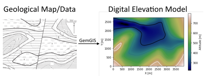
Creating Digital Elevation Model from Contour Lines#
The digital elevation model (DEM) will be created by interpolating contour lines digitized from the georeferenced map using the SciPy Radial Basis Function interpolation wrapped in GemGIS. The respective function used for that is gg.vector.interpolate_raster().
[5]:
import matplotlib.pyplot as plt
import matplotlib.image as mpimg
img = mpimg.imread('../images/dem_example18.png')
plt.figure(figsize=(10, 10))
imgplot = plt.imshow(img)
plt.axis('off')
plt.tight_layout()
[6]:
topo = gpd.read_file(file_path + 'topo18.shp')
topo.head()
[6]:
| id | Z | geometry | |
|---|---|---|---|
| 0 | None | 700 | LINESTRING (3.286 332.303, 62.614 304.560, 120... |
| 1 | None | 700 | LINESTRING (27.188 946.063, 60.480 983.196, 98... |
| 2 | None | 500 | LINESTRING (1024.228 2750.211, 1101.055 2721.1... |
| 3 | None | 400 | LINESTRING (317.849 2757.466, 375.042 2739.113... |
| 4 | None | 300 | LINESTRING (4.567 2715.638, 60.480 2702.407, 1... |
Interpolating the contour lines#
[7]:
topo_raster = gg.vector.interpolate_raster(gdf=topo, value='Z', method='rbf', res=10)
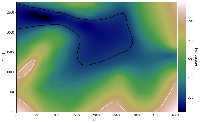
Plotting the raster#
[8]:
import matplotlib.pyplot as plt

from mpl_toolkits.axes_grid1 import make_axes_locatable
fix, ax = plt.subplots(1, figsize=(10, 10))
topo.plot(ax=ax, aspect='equal', column='Z', cmap='gist_earth')
im = plt.imshow(topo_raster, origin='lower', extent=[0, 4022, 0, 2761], cmap='gist_earth')
divider = make_axes_locatable(ax)
cax = divider.append_axes("right", size="5%", pad=0.05)
cbar = plt.colorbar(im, cax=cax)
cbar.set_label('Altitude [m]')
ax.set_xlabel('X [m]')
ax.set_ylabel('Y [m]')
ax.set_xlim(0, 4022)
ax.set_ylim(0, 2761)
[8]:
(0.0, 2761.0)
Saving the raster to disc#
After the interpolation of the contour lines, the raster is saved to disc using gg.raster.save_as_tiff(). The function will not be executed as a raster is already provided with the example data.
Opening Raster#
The previously computed and saved raster can now be opened using rasterio.
[9]:
topo_raster = rasterio.open(file_path + 'raster18.tif')
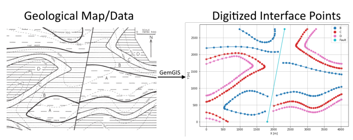
Interface Points of stratigraphic boundaries#
The interface points will be extracted from LineStrings digitized from the georeferenced map using QGIS. It is important to provide a formation name for each layer boundary. The vertical position of the interface point will be extracted from the digital elevation model using the GemGIS function gg.vector.extract_xyz(). The resulting GeoDataFrame now contains single points including the information about the respective formation.
[10]:
import matplotlib.pyplot as plt
import matplotlib.image as mpimg
img = mpimg.imread('../images/interfaces_example18.png')
plt.figure(figsize=(10, 10))
imgplot = plt.imshow(img)
plt.axis('off')
plt.tight_layout()
[11]:
interfaces = gpd.read_file(file_path + 'interfaces18.shp')
interfaces.head()
[11]:
| id | formation | geometry | |
|---|---|---|---|
| 0 | None | Fault | LINESTRING (2326.868 2757.893, 1812.982 1.522) |
| 1 | None | D | LINESTRING (4.567 1721.586, 117.246 1763.414, ... |
| 2 | None | C | LINESTRING (3.713 1860.728, 129.197 1896.580, ... |
| 3 | None | C | LINESTRING (4.140 279.378, 100.600 258.891, 20... |
| 4 | None | D | LINESTRING (4.140 101.823, 100.600 92.433, 196... |
Extracting Z coordinate from Digital Elevation Model#
[12]:
interfaces_coords = gg.vector.extract_xyz(gdf=interfaces, dem=topo_raster)
interfaces_coords = interfaces_coords.sort_values(by='formation', ascending=False)
interfaces_coords = interfaces_coords[interfaces_coords['formation'].isin(['Fault', 'D', 'C', 'B'])]
interfaces_coords.head()
[12]:
| formation | geometry | X | Y | Z | |
|---|---|---|---|---|---|
| 0 | Fault | POINT (2326.868 2757.893) | 2326.87 | 2757.89 | 396.78 |
| 1 | Fault | POINT (1812.982 1.522) | 1812.98 | 1.52 | 645.29 |
| 263 | D | POINT (3437.014 1929.018) | 3437.01 | 1929.02 | 488.43 |
| 256 | D | POINT (3007.638 2177.425) | 3007.64 | 2177.42 | 371.88 |
| 257 | D | POINT (3057.575 2147.121) | 3057.57 | 2147.12 | 390.98 |
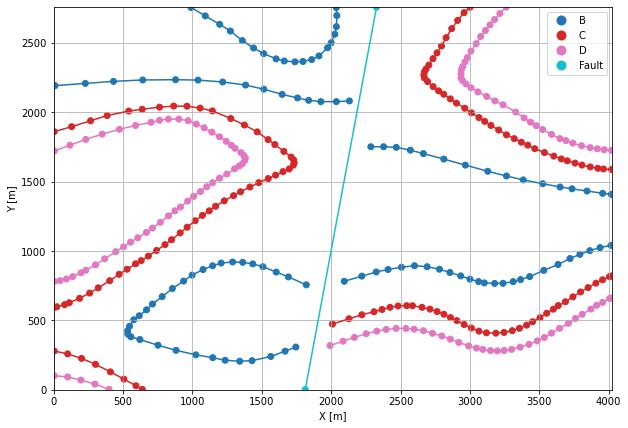
Plotting the Interface Points#
[13]:
fig, ax = plt.subplots(1, figsize=(10, 10))

interfaces.plot(ax=ax, column='formation', legend=True, aspect='equal')
interfaces_coords.plot(ax=ax, column='formation', legend=True, aspect='equal')
plt.grid()
ax.set_xlabel('X [m]')
ax.set_ylabel('Y [m]')
ax.set_xlim(0, 4022)
ax.set_ylim(0, 2761)
[13]:
(0.0, 2761.0)
Orientations from Strike Lines#
Strike lines connect outcropping stratigraphic boundaries (interfaces) of the same altitude. In other words: the intersections between topographic contours and stratigraphic boundaries at the surface. The height difference and the horizontal difference between two digitized lines is used to calculate the dip and azimuth and hence an orientation that is necessary for GemPy. In order to calculate the orientations, each set of strikes lines/LineStrings for one formation must be given an id
number next to the altitude of the strike line. The id field is already predefined in QGIS. The strike line with the lowest altitude gets the id number 1, the strike line with the highest altitude the the number according to the number of digitized strike lines. It is currently recommended to use one set of strike lines for each structural element of one formation as illustrated.
[14]:
import matplotlib.pyplot as plt
import matplotlib.image as mpimg
img = mpimg.imread('../images/orientations_example18.png')
plt.figure(figsize=(10, 10))
imgplot = plt.imshow(img)
plt.axis('off')
plt.tight_layout()
[15]:
strikes = gpd.read_file(file_path + 'strikes18.shp')
strikes.head()
[15]:
| id | formation | Z | geometry | |
|---|---|---|---|---|
| 0 | 1 | C2 | 300 | LINESTRING (2391.317 2132.396, 2809.062 2132.076) |
| 1 | 2 | C2 | 400 | LINESTRING (2334.977 1895.513, 3168.227 1897.754) |
| 2 | 3 | C2 | 500 | LINESTRING (3747.308 1638.464, 2608.992 1647.107) |
| 3 | 1 | D2 | 400 | LINESTRING (2393.237 2137.518, 3072.514 2137.838) |
| 4 | 2 | D2 | 500 | LINESTRING (2273.516 1895.513, 3486.738 1900.315) |
Calculate Orientations for each formation#
[16]:
orientations_d1 = gg.vector.calculate_orientations_from_strike_lines(gdf=strikes[strikes['formation'] == 'D1'].sort_values(by='Z', ascending=True).reset_index())
orientations_d1
[16]:
| dip | azimuth | Z | geometry | polarity | formation | X | Y | |
|---|---|---|---|---|---|---|---|---|
| 0 | 21.76 | 180.11 | 650.00 | POINT (2901.894 492.786) | 1.00 | D1 | 2901.89 | 492.79 |
[17]:
orientations_d2 = gg.vector.calculate_orientations_from_strike_lines(gdf=strikes[strikes['formation'] == 'D2'].sort_values(by='Z', ascending=True).reset_index())
orientations_d2
[17]:
| dip | azimuth | Z | geometry | polarity | formation | X | Y | |
|---|---|---|---|---|---|---|---|---|
| 0 | 22.69 | 359.82 | 450.00 | POINT (2806.501 2017.796) | 1.00 | D2 | 2806.50 | 2017.80 |
[18]:
orientations_d3 = gg.vector.calculate_orientations_from_strike_lines(gdf=strikes[strikes['formation'] == 'D3'].sort_values(by='Z', ascending=True).reset_index())
orientations_d3
[18]:
| dip | azimuth | Z | geometry | polarity | formation | X | Y | |
|---|---|---|---|---|---|---|---|---|
| 0 | 0.00 | 0.00 | 400.00 | POINT (645.350 1647.827) | 1.00 | D3 | 645.35 | 1647.83 |
| 1 | 21.14 | 0.41 | 450.00 | POINT (507.462 1396.780) | 1.00 | D3 | 507.46 | 1396.78 |
| 2 | 21.96 | 359.46 | 550.00 | POINT (333.881 1138.690) | 1.00 | D3 | 333.88 | 1138.69 |
[19]:
orientations_d4 = gg.vector.calculate_orientations_from_strike_lines(gdf=strikes[strikes['formation'] == 'D4'].sort_values(by='Z', ascending=True).reset_index())
orientations_d4
[19]:
| dip | azimuth | Z | geometry | polarity | formation | X | Y | |
|---|---|---|---|---|---|---|---|---|
| 0 | 21.86 | 180.50 | 450.00 | POINT (2683.258 2522.931) | 1.00 | D4 | 2683.26 | 2522.93 |
[20]:
orientations_c1 = gg.vector.calculate_orientations_from_strike_lines(gdf=strikes[strikes['formation'] == 'C1'].sort_values(by='Z', ascending=True).reset_index())
orientations_c1
[20]:
| dip | azimuth | Z | geometry | polarity | formation | X | Y | |
|---|---|---|---|---|---|---|---|---|
| 0 | 22.06 | 180.54 | 350.00 | POINT (865.026 1893.753) | 1.00 | C1 | 865.03 | 1893.75 |
[21]:
orientations_c2 = gg.vector.calculate_orientations_from_strike_lines(gdf=strikes[strikes['formation'] == 'C2'].sort_values(by='Z', ascending=True).reset_index())
orientations_c2
[21]:
| dip | azimuth | Z | geometry | polarity | formation | X | Y | |
|---|---|---|---|---|---|---|---|---|
| 0 | 23.03 | 359.89 | 350.00 | POINT (2675.896 2014.435) | 1.00 | C2 | 2675.90 | 2014.43 |
| 1 | 21.87 | 0.23 | 450.00 | POINT (2964.876 1769.710) | 1.00 | C2 | 2964.88 | 1769.71 |
[22]:
orientations_c3 = gg.vector.calculate_orientations_from_strike_lines(gdf=strikes[strikes['formation'] == 'C3'].sort_values(by='Z', ascending=True).reset_index())
orientations_c3
[22]:
| dip | azimuth | Z | geometry | polarity | formation | X | Y | |
|---|---|---|---|---|---|---|---|---|
| 0 | 0.00 | 0.32 | 300.00 | POINT (812.528 1648.067) | 1.00 | C3 | 812.53 | 1648.07 |
| 1 | 11.14 | 359.66 | 350.00 | POINT (699.208 1512.340) | 1.00 | C3 | 699.21 | 1512.34 |
| 2 | 23.45 | 359.84 | 450.00 | POINT (459.445 1139.411) | 1.00 | C3 | 459.45 | 1139.41 |
| 3 | 20.58 | 180.00 | 550.00 | POINT (278.262 889.083) | 1.00 | C3 | 278.26 | 889.08 |
[23]:
orientations_c4 = gg.vector.calculate_orientations_from_strike_lines(gdf=strikes[strikes['formation'] == 'C4'].sort_values(by='Z', ascending=True).reset_index())
orientations_c4
[23]:
| dip | azimuth | Z | geometry | polarity | formation | X | Y | |
|---|---|---|---|---|---|---|---|---|
| 0 | 21.54 | 180.38 | 350.00 | POINT (2575.061 2523.892) | 1.00 | C4 | 2575.06 | 2523.89 |
[24]:
orientations_c5 = gg.vector.calculate_orientations_from_strike_lines(gdf=strikes[strikes['formation'] == 'C5'].sort_values(by='Z', ascending=True).reset_index())
orientations_c5
[24]:
| dip | azimuth | Z | geometry | polarity | formation | X | Y | |
|---|---|---|---|---|---|---|---|---|
| 0 | 23.45 | 180.08 | 650.00 | POINT (1102.869 125.938) | 1.00 | C5 | 1102.87 | 125.94 |
[25]:
orientations_b1 = gg.vector.calculate_orientations_from_strike_lines(gdf=strikes[strikes['formation'] == 'B1'].sort_values(by='Z', ascending=True).reset_index())
orientations_b1
[25]:
| dip | azimuth | Z | geometry | polarity | formation | X | Y | |
|---|---|---|---|---|---|---|---|---|
| 0 | 24.55 | 180.05 | 450.00 | POINT (1590.398 2647.615) | 1.00 | B1 | 1590.40 | 2647.61 |
[26]:
orientations_b2 = gg.vector.calculate_orientations_from_strike_lines(gdf=strikes[strikes['formation'] == 'B2'].sort_values(by='Z', ascending=True).reset_index())
orientations_b2
[26]:
| dip | azimuth | Z | geometry | polarity | formation | X | Y | |
|---|---|---|---|---|---|---|---|---|
| 0 | 11.29 | 0.26 | 450.00 | POINT (1321.745 502.309) | 1.00 | B2 | 1321.74 | 502.31 |
[27]:
orientations_fault = gpd.read_file(file_path + 'orientations18_fault.shp')
orientations_fault = gg.vector.extract_xyz(gdf=orientations_fault, dem=topo_raster)
orientations_fault
[27]:
| formation | dip | azimuth | polarity | geometry | X | Y | Z | |
|---|---|---|---|---|---|---|---|---|
| 0 | Fault | 90.00 | 280.00 | 1.00 | POINT (1918.192 566.731) | 1918.19 | 566.73 | 490.30 |
| 1 | Fault | 90.00 | 280.00 | 1.00 | POINT (2190.927 2031.561) | 2190.93 | 2031.56 | 255.41 |
Merging Orientations#
[28]:
import pandas as pd
orientations = pd.concat([orientations_fault, orientations_d1, orientations_d2, orientations_d3, orientations_d4, orientations_c1, orientations_c2, orientations_c3[:-1], orientations_c4, orientations_c5, orientations_b1, orientations_b2]).reset_index()
orientations['formation'] = ['Fault', 'Fault', 'D', 'D', 'D', 'D', 'D', 'D', 'C', 'C', 'C', 'C', 'C', 'C', 'C', 'C', 'B', 'B']
orientations = orientations[orientations['formation'].isin(['Fault', 'D', 'C', 'B'])]
orientations
[28]:
| index | formation | dip | azimuth | polarity | geometry | X | Y | Z | |
|---|---|---|---|---|---|---|---|---|---|
| 0 | 0 | Fault | 90.00 | 280.00 | 1.00 | POINT (1918.192 566.731) | 1918.19 | 566.73 | 490.30 |
| 1 | 1 | Fault | 90.00 | 280.00 | 1.00 | POINT (2190.927 2031.561) | 2190.93 | 2031.56 | 255.41 |
| 2 | 0 | D | 21.76 | 180.11 | 1.00 | POINT (2901.894 492.786) | 2901.89 | 492.79 | 650.00 |
| 3 | 0 | D | 22.69 | 359.82 | 1.00 | POINT (2806.501 2017.796) | 2806.50 | 2017.80 | 450.00 |
| 4 | 0 | D | 0.00 | 0.00 | 1.00 | POINT (645.350 1647.827) | 645.35 | 1647.83 | 400.00 |
| 5 | 1 | D | 21.14 | 0.41 | 1.00 | POINT (507.462 1396.780) | 507.46 | 1396.78 | 450.00 |
| 6 | 2 | D | 21.96 | 359.46 | 1.00 | POINT (333.881 1138.690) | 333.88 | 1138.69 | 550.00 |
| 7 | 0 | D | 21.86 | 180.50 | 1.00 | POINT (2683.258 2522.931) | 2683.26 | 2522.93 | 450.00 |
| 8 | 0 | C | 22.06 | 180.54 | 1.00 | POINT (865.026 1893.753) | 865.03 | 1893.75 | 350.00 |
| 9 | 0 | C | 23.03 | 359.89 | 1.00 | POINT (2675.896 2014.435) | 2675.90 | 2014.43 | 350.00 |
| 10 | 1 | C | 21.87 | 0.23 | 1.00 | POINT (2964.876 1769.710) | 2964.88 | 1769.71 | 450.00 |
| 11 | 0 | C | 0.00 | 0.32 | 1.00 | POINT (812.528 1648.067) | 812.53 | 1648.07 | 300.00 |
| 12 | 1 | C | 11.14 | 359.66 | 1.00 | POINT (699.208 1512.340) | 699.21 | 1512.34 | 350.00 |
| 13 | 2 | C | 23.45 | 359.84 | 1.00 | POINT (459.445 1139.411) | 459.45 | 1139.41 | 450.00 |
| 14 | 0 | C | 21.54 | 180.38 | 1.00 | POINT (2575.061 2523.892) | 2575.06 | 2523.89 | 350.00 |
| 15 | 0 | C | 23.45 | 180.08 | 1.00 | POINT (1102.869 125.938) | 1102.87 | 125.94 | 650.00 |
| 16 | 0 | B | 24.55 | 180.05 | 1.00 | POINT (1590.398 2647.615) | 1590.40 | 2647.61 | 450.00 |
| 17 | 0 | B | 11.29 | 0.26 | 1.00 | POINT (1321.745 502.309) | 1321.74 | 502.31 | 450.00 |
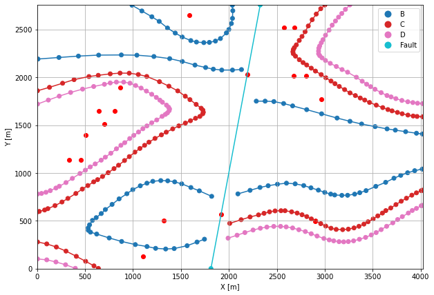
Plotting the Orientations#
[29]:
fig, ax = plt.subplots(1, figsize=(10, 10))

interfaces.plot(ax=ax, column='formation', legend=True, aspect='equal')
interfaces_coords.plot(ax=ax, column='formation', legend=True, aspect='equal')
orientations.plot(ax=ax, color='red', aspect='equal')
plt.grid()
ax.set_xlabel('X [m]')
ax.set_ylabel('Y [m]')
ax.set_xlim(0, 4022)
ax.set_ylim(0, 2761)
[29]:
(0.0, 2761.0)
GemPy Model Construction#
The structural geological model will be constructed using the GemPy package.
[30]:
import gempy as gp
WARNING (theano.configdefaults): g++ not available, if using conda: `conda install m2w64-toolchain`
WARNING (theano.configdefaults): g++ not detected ! Theano will be unable to execute optimized C-implementations (for both CPU and GPU) and will default to Python implementations. Performance will be severely degraded. To remove this warning, set Theano flags cxx to an empty string.
WARNING (theano.tensor.blas): Using NumPy C-API based implementation for BLAS functions.
Creating new Model#
[31]:
geo_model = gp.create_model('Model18')
geo_model
[31]:
Model18 2022-04-05 11:12
Initiate Data#
[32]:
gp.init_data(geo_model, [0, 4022, 0, 2761, 0, 1000], [100, 100, 100],
             surface_points_df=interfaces_coords[interfaces_coords['Z'] != 0],
             orientations_df=orientations,
             default_values=True)
Active grids: ['regular']
[32]:
Model18 2022-04-05 11:12
Model Surfaces#
[33]:
geo_model.surfaces
[33]:
| surface | series | order_surfaces | color | id | |
|---|---|---|---|---|---|
| 0 | Fault | Default series | 1 | #015482 | 1 |
| 1 | D | Default series | 2 | #9f0052 | 2 |
| 2 | C | Default series | 3 | #ffbe00 | 3 |
| 3 | B | Default series | 4 | #728f02 | 4 |
Mapping the Stack to Surfaces#
[34]:
gp.map_stack_to_surfaces(geo_model,
                         {
                          'Fault1': ('Fault'),
                          'Strata1': ('D', 'C', 'B'),
                         },
                         remove_unused_series=True)
geo_model.add_surfaces('A')
geo_model.set_is_fault(['Fault1'])
Fault colors changed. If you do not like this behavior, set change_color to False.
[34]:
| order_series | BottomRelation | isActive | isFault | isFinite | |
|---|---|---|---|---|---|
| Fault1 | 1 | Fault | True | True | False |
| Strata1 | 2 | Erosion | True | False | False |
Showing the Number of Data Points#
[35]:
gg.utils.show_number_of_data_points(geo_model=geo_model)
[35]:
| surface | series | order_surfaces | color | id | No. of Interfaces | No. of Orientations | |
|---|---|---|---|---|---|---|---|
| 0 | Fault | Fault1 | 1 | #527682 | 1 | 2 | 2 |
| 1 | D | Strata1 | 1 | #9f0052 | 2 | 125 | 6 |
| 2 | C | Strata1 | 2 | #ffbe00 | 3 | 137 | 8 |
| 3 | B | Strata1 | 3 | #728f02 | 4 | 108 | 2 |
| 4 | A | Strata1 | 4 | #443988 | 5 | 0 | 0 |
Loading Digital Elevation Model#
[36]:
geo_model.set_topography(
    source='gdal', filepath=file_path + 'raster18.tif')
Cropped raster to geo_model.grid.extent.
depending on the size of the raster, this can take a while...
storing converted file...
Active grids: ['regular' 'topography']
[36]:
Grid Object. Values:
array([[  20.11      ,   13.805     ,    5.        ],
       [  20.11      ,   13.805     ,   15.        ],
       [  20.11      ,   13.805     ,   25.        ],
       ...,
       [4016.99751244, 2735.99094203,  715.64483643],
       [4016.99751244, 2745.99456522,  716.50982666],
       [4016.99751244, 2755.99818841,  717.38183594]])
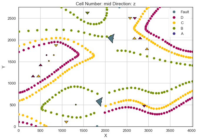
Plotting Input Data#
[37]:
gp.plot_2d(geo_model, direction='z', show_lith=False, show_boundaries=False)
plt.grid()
[38]:
gp.plot_3d(geo_model, image=False, plotter_type='basic', notebook=True)
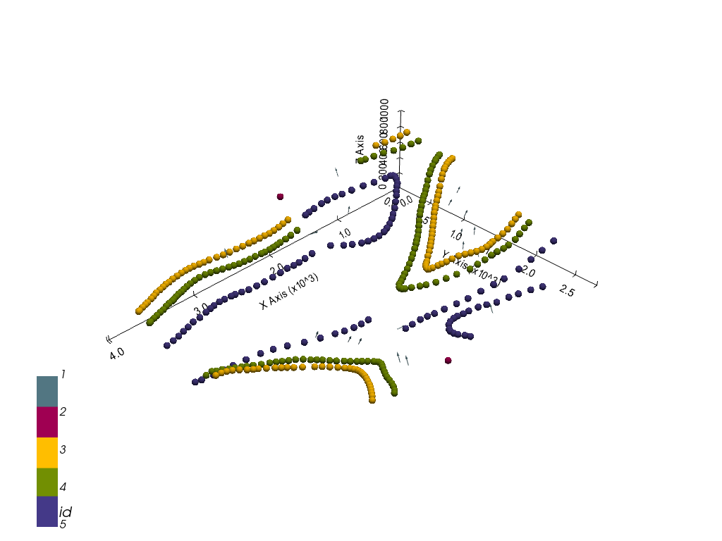
[38]:
<gempy.plot.vista.GemPyToVista at 0x1e57957d130>
Setting the Interpolator#
[39]:
gp.set_interpolator(geo_model,
                    compile_theano=True,
                    theano_optimizer='fast_compile',
                    verbose=[],
                    update_kriging=False
                    )
Compiling theano function...
Level of Optimization:  fast_compile
Device:  cpu
Precision:  float64
Number of faults:  1
Compilation Done!
Kriging values:
                    values
range             4979.92
$C_o$           590466.79
drift equations    [3, 3]
[39]:
<gempy.core.interpolator.InterpolatorModel at 0x1e578a9eb20>
Computing Model#
[40]:
sol = gp.compute_model(geo_model, compute_mesh=True)
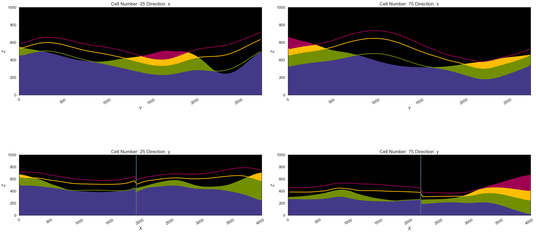
Plotting Cross Sections#
[41]:
gp.plot_2d(geo_model, direction=['x', 'x', 'y', 'y'], cell_number=[25, 75, 25, 75], show_topography=True, show_data=False)
[41]:
<gempy.plot.visualization_2d.Plot2D at 0x1e57c2d2d90>
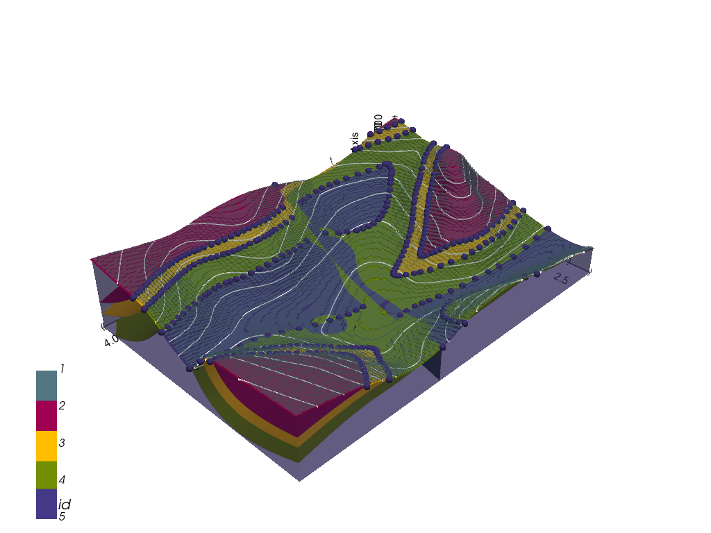
Plotting 3D Model#
[42]:
gpv = gp.plot_3d(geo_model, image=False, show_topography=True,
                 plotter_type='basic', notebook=True, show_lith=True)
[ ]: