01 Extract XY Coordinates#

Vector data is commonly provided as shape files. These files can be loaded with GeoPandas as GeoDataFrames. Each geometry object is stored as shapely object within the GeoSeries geometry of the GeoDataFrames. The basic shapely objects, also called Base Geometries, used here are:

Points/Multi-Points
Lines/Multi-Lines
Polygons/Multi-Polygons
Geometry Collections

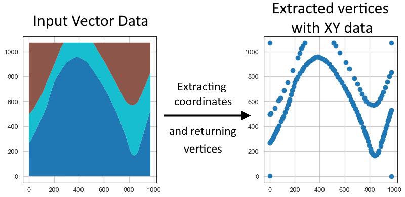
The first step is to load the data using GeoPandas. We can inspect the different columns of the GeoDataFrame by looking at its head. In the following examples for point, line and polygon data, we have an id column which was created during the digitalizing of the data in QGIS, a formation column containing the name of a geological unit (this becomes important later for the actual modeling) and most importantly the geometry column consisting of the shapely geometry objects. The X and Y coordinates of the different geometry objects can then be extracted using extract_xy() of the GemGIS vector module.

c8720a0299224886a76595a8b2a3d276

Set File Paths and download Tutorial Data#

If you downloaded the latest GemGIS version from the Github repository, append the path so that the package can be imported successfully. Otherwise, it is recommended to install GemGIS via pip install gemgis and import GemGIS using import gemgis as gg. In addition, the file path to the folder where the data is being stored is set. The tutorial data is downloaded using Pooch (https://www.fatiando.org/pooch/latest/index.html) and stored in the specified folder. Use pip install pooch if Pooch is not installed on your system yet.

[1]:

import gemgis as gg

file_path ='data/01_extract_xy/'

[2]:

gg.download_gemgis_data.download_tutorial_data(filename="01_extract_xy.zip", dirpath=file_path)

Downloading file '01_extract_xy.zip' from 'https://rwth-aachen.sciebo.de/s/AfXRsZywYDbUF34/download?path=%2F01_extract_xy.zip' to 'C:\Users\ale93371\Documents\gemgis\docs\getting_started\tutorial\data\01_extract_xy'.

Point Data#

The point data stored as shape file will be loaded as GeoDataFrame. It contains an id, formation and the geometry column.

[3]:

import geopandas as gpd

gdf = gpd.read_file(file_path + 'interfaces_points.shp')

gdf.head()

[3]:

	id	formation	geometry
0	None	Ton	POINT (19.15013 293.31349)
1	None	Ton	POINT (61.93437 381.45933)
2	None	Ton	POINT (109.35786 480.94557)
3	None	Ton	POINT (157.81230 615.99943)
4	None	Ton	POINT (191.31803 719.09398)

Inspecting the geometry column#

The elements of the geometry columns can be accessed by indexing the GeoDataFrame. It can be seen that the objects in the geometry column are Shapely objects.

[4]:

gdf.loc[0].geometry

[4]:

../../_images/getting_started_tutorial_01_extract_xy_7_0.svg

[5]:

gdf.loc[0].geometry.wkt

[5]:

'POINT (19.150128045807676 293.313485355882)'

[6]:

type(gdf.loc[0].geometry)

[6]:

shapely.geometry.point.Point

Extracting the Coordinates#

The resulting GeoDataFrame has now an additional X and Y column containing the coordinates of the point objects. These can now be easily used for further processing. The geometry types of the shapely objects remained unchanged. The id column was dropped by default.

[7]:

gdf_xy = gg.vector.extract_xy(gdf=gdf)

gdf_xy.head()

[7]:

	formation	geometry	X	Y
0	Ton	POINT (19.15013 293.31349)	19.15	293.31
1	Ton	POINT (61.93437 381.45933)	61.93	381.46
2	Ton	POINT (109.35786 480.94557)	109.36	480.95
3	Ton	POINT (157.81230 615.99943)	157.81	616.00
4	Ton	POINT (191.31803 719.09398)	191.32	719.09

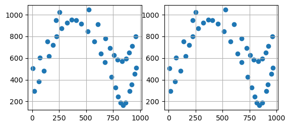
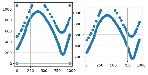
Plotting the Data#

The figures below show the original point data and the extracted X and Y data using matplotlib.

[8]:

import matplotlib.pyplot as plt

fig, (ax1,ax2) = plt.subplots(1,2)

gdf.plot(ax=ax1, aspect='equal')
ax1.grid()

gdf_xy.plot(ax=ax2, aspect='equal')
ax2.grid()

../../_images/getting_started_tutorial_01_extract_xy_13_0.png

Line Data#

The line data stored as shape file will be loaded as GeoDataFrame. It consists of the same columns as the shape file containing points.

[9]:

import geopandas as gpd
import gemgis as gg

gdf = gpd.read_file(file_path + 'interfaces_lines.shp')

gdf.head()

[9]:

	id	formation	geometry
0	None	Sand1	LINESTRING (0.25633 264.86215, 10.59347 276.73...
1	None	Ton	LINESTRING (0.18819 495.78721, 8.84067 504.141...
2	None	Ton	LINESTRING (970.67663 833.05262, 959.37243 800...

Inspecting the geometry column#

The elements of the geometry columns can be accessed by indexing the GeoDataFrame. It can be seen that the objects in the geometry column are Shapely objects.

[10]:

gdf.loc[0].geometry

[10]:

../../_images/getting_started_tutorial_01_extract_xy_17_0.svg

[11]:

gdf.loc[0].geometry.wkt[:100]

[11]:

'LINESTRING (0.256327195431048 264.86214748436396, 10.59346813871597 276.73370778641777, 17.134940141'

[12]:

type(gdf.loc[0].geometry)

[12]:

shapely.geometry.linestring.LineString

Extracting the Coordinates to Point Objects#

The resulting GeoDataFrame has now an additional X and Y column. These values represent the single vertices of each LineString. The geometry types of the shapely objects in the GeoDataFrame were converted from LineStrings to Points to match the X and Y column data. The id column was dropped by default. The index of the new GeoDataFrame was reset.

[13]:

gdf_xy = gg.vector.extract_xy(gdf=gdf)

gdf_xy.head()

[13]:

	formation	geometry	X	Y
0	Sand1	POINT (0.25633 264.86215)	0.26	264.86
1	Sand1	POINT (10.59347 276.73371)	10.59	276.73
2	Sand1	POINT (17.13494 289.08982)	17.13	289.09
3	Sand1	POINT (19.15013 293.31349)	19.15	293.31
4	Sand1	POINT (27.79512 310.57169)	27.80	310.57

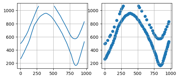
Plotting the Data#

The figures below show the original line data and the extracted point data with the respective X and Y data using matplotlib. It can be seen that the single vertices the original LineStrings were made of were extracted.

[14]:

import matplotlib.pyplot as plt

fig, (ax1,ax2) = plt.subplots(1,2)

gdf.plot(ax=ax1, aspect='equal')
ax1.grid()

gdf_xy.plot(ax=ax2, aspect='equal')
ax2.grid()

../../_images/getting_started_tutorial_01_extract_xy_23_0.png

Extracting the Coordinates to list of X and Y coordinates in separate cells#

The coordinates of LineStrings in a GeoDataFrame can also be extracted and are stored as lists in respective X and Y columns using extract_xy_linestring(..).

[15]:

gdf_xy = gg.vector.extract_xy_linestring(gdf=gdf)
gdf_xy

[15]:

	id	formation	geometry	X	Y
0	None	Sand1	LINESTRING (0.25633 264.86215, 10.59347 276.73...	[0.256327195431048, 10.59346813871597, 17.1349...	[264.86214748436396, 276.73370778641777, 289.0...
1	None	Ton	LINESTRING (0.18819 495.78721, 8.84067 504.141...	[0.1881868620686138, 8.840672956663411, 41.092...	[495.787213546976, 504.1418419288791, 546.4230...
2	None	Ton	LINESTRING (970.67663 833.05262, 959.37243 800...	[970.6766251230017, 959.3724321757514, 941.291...	[833.052616499831, 800.0232029873156, 754.8012...

Polygon Data#

The polygon data stored as shape file will be loaded as GeoDataFrame. It can be seen that the objects in the geometry column are Shapely objects.

[16]:

import geopandas as gpd
import gemgis as gg

gdf = gpd.read_file(file_path + 'interfaces_polygons.shp')

gdf.head()

[16]:

	id	formation	geometry
0	None	Sand1	POLYGON ((0.25633 264.86215, 10.59347 276.7337...
1	None	Ton	POLYGON ((0.25633 264.86215, 0.18819 495.78721...
2	None	Sand2	POLYGON ((0.18819 495.78721, 0.24897 1068.7595...
3	None	Sand2	POLYGON ((511.67477 1068.85246, 971.69794 1068...

Inspecting the geometry column#

The elements of the geometry columns can be accessed by indexing the GeoDataFrame. It can be seen that the objects in the geometry column are Shapely objects.

[17]:

gdf.loc[0].geometry

[17]:

../../_images/getting_started_tutorial_01_extract_xy_29_0.svg

[18]:

gdf.loc[0].geometry.wkt[:100]

[18]:

'POLYGON ((0.256327195431048 264.86214748436396, 10.59346813871597 276.73370778641777, 17.13494014188'

[19]:

type(gdf.loc[0].geometry)

[19]:

shapely.geometry.polygon.Polygon

Extracting the Coordinates#

The resulting GeoDataFrame has now an additional X and Y column. These values represent the single vertices of each Polygon. The geometry types of the shapely objects in the GeoDataFrame were converted from Polygons to Points to match the X and Y column data. The id column was dropped by default. The index of the new GeoDataFrame was reset.

[20]:

gdf_xy = gg.vector.extract_xy(gdf=gdf)

gdf_xy.head()

[20]:

	formation	geometry	X	Y
0	Sand1	POINT (0.25633 264.86215)	0.26	264.86
1	Sand1	POINT (10.59347 276.73371)	10.59	276.73
2	Sand1	POINT (17.13494 289.08982)	17.13	289.09
3	Sand1	POINT (19.15013 293.31349)	19.15	293.31
4	Sand1	POINT (27.79512 310.57169)	27.80	310.57

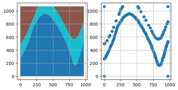
Plotting the Data#

The figures below show the original polygon data and the extracted point data with the respective X and Y data using matplotlib. It can be seen that the single vertices the original Polygons were made of were extracted.

[21]:

import matplotlib.pyplot as plt

fig, (ax1,ax2) = plt.subplots(1,2)

gdf.plot(ax=ax1, column='formation', aspect='equal')
ax1.grid()

gdf_xy.plot(ax=ax2, aspect='equal')
ax2.grid()

../../_images/getting_started_tutorial_01_extract_xy_35_0.png

Removing the corner points of the polygons#

In the above plot, it can be seen, that the corner points are still present in the extracted X and Y point pairs. The additional argument remove_total_bounds can be used to remove vertices that are equal to either of the total bounds of the polygon gdf.

The total bounds of the original gdf:

[22]:

gdf.total_bounds

[22]:

array([ 1.88186862e-01, -6.89945891e-03,  9.72088904e+02,  1.06885246e+03])

The length of the extracted vertices:

[23]:

len(gdf_xy)

[23]:

Extracting the vertices but removing the total bounds. A total of 18 points were removed that were within 0.1 units of the total bounds.

[24]:

gdf_xy_without_bounds = gg.vector.extract_xy(gdf=gdf, remove_total_bounds=True, threshold_bounds=0.1)
print(len(gdf_xy_without_bounds))
gdf_xy_without_bounds.head()

[24]:

	formation	geometry	X	Y
1	Sand1	POINT (10.59347 276.73371)	10.59	276.73
2	Sand1	POINT (17.13494 289.08982)	17.13	289.09
3	Sand1	POINT (19.15013 293.31349)	19.15	293.31
4	Sand1	POINT (27.79512 310.57169)	27.80	310.57
5	Sand1	POINT (34.41735 324.13919)	34.42	324.14

The removal of the points can also be inspected visually.

[25]:

import matplotlib.pyplot as plt

fig, (ax1,ax2) = plt.subplots(1,2)

gdf_xy.plot(ax=ax1, aspect='equal')
ax1.grid()

gdf_xy_without_bounds.plot(ax=ax2, aspect='equal')
ax2.grid()

../../_images/getting_started_tutorial_01_extract_xy_43_0.png

Geometry Collections#

Geometry collections contain different types of geometries. Here, a GeoDataFrame is created with one GeometryCollection object and two LineStrings.

[26]:

from shapely.geometry import LineString
import geopandas as gpd
import gemgis as gg

line1 = LineString([(0, 0), (1, 1), (1, 2), (2, 2)])
line2 = LineString([(0, 0), (1, 1), (2, 1), (2, 2)])
collection = line1.intersection(line2)

[27]:

type(collection)

[27]:

shapely.geometry.collection.GeometryCollection

Creating the GeoDataFrame with different geom_types#

[28]:

gdf = gpd.GeoDataFrame(geometry=[collection, line1, line2])
gdf

[28]:

	geometry
0	GEOMETRYCOLLECTION (LINESTRING (0.00000 0.0000...
1	LINESTRING (0.00000 0.00000, 1.00000 1.00000, ...
2	LINESTRING (0.00000 0.00000, 1.00000 1.00000, ...

Extracting the Coordinates#

NB: By default, points within a geometry collection are dropped as they usually do not represent true layer boundaries and rather corner points.

[29]:

gdf_xy = gg.vector.extract_xy(gdf=gdf)

gdf_xy

[29]:

	geometry	X	Y
0	POINT (0.00000 0.00000)	0.00	0.00
1	POINT (1.00000 1.00000)	1.00	1.00
2	POINT (0.00000 0.00000)	0.00	0.00
3	POINT (1.00000 1.00000)	1.00	1.00
4	POINT (1.00000 2.00000)	1.00	2.00
5	POINT (2.00000 2.00000)	2.00	2.00
6	POINT (0.00000 0.00000)	0.00	0.00
7	POINT (1.00000 1.00000)	1.00	1.00
8	POINT (2.00000 1.00000)	2.00	1.00
9	POINT (2.00000 2.00000)	2.00	2.00

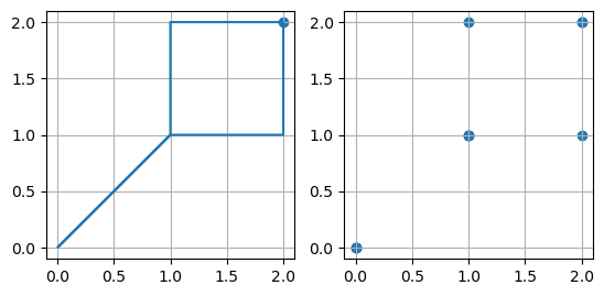
Plotting the Data#

The figures below show the original polygon data and the extracted point data with the respective X and Y data with matplotlib. Note the point in the upper right of the left plot which was dropped during the extraction of the vertices.

[30]:

import matplotlib.pyplot as plt

fig, (ax1,ax2) = plt.subplots(1,2)

gdf.plot(ax=ax1, aspect='equal')
ax1.grid()

gdf_xy.plot(ax=ax2, aspect='equal')
ax2.grid()

../../_images/getting_started_tutorial_01_extract_xy_52_0.png

Additional Arguments#

Several additional arguments can be passed to adapt the functionality of the function. For further reference, see the API Reference for extract_xy.

reset_index (bool)
drop_id (bool)
drop_level0 (bool)
drop_level1 (bool)
drop_index (bool)
drop_points (bool)
overwrite_xy (bool)
target_crs(str, pyproj.crs.crs.CRS)
bbox (list)
remove_total_bounds (bool)
threshold_bounds (float, int)

Original Function#

Original function with default values of arguments.

[31]:

gdf_xy = gg.vector.extract_xy(gdf=gdf,
                              reset_index=True,
                              drop_id=True,
                              drop_level0=True,
                              drop_level1=True,
                              drop_index=True,
                              drop_points=True,
                              overwrite_xy=True,
                              target_crs=gdf.crs,
                              bbox = None)

gdf_xy.head()

[31]:

	geometry	X	Y
0	POINT (0.00000 0.00000)	0.00	0.00
1	POINT (1.00000 1.00000)	1.00	1.00
2	POINT (0.00000 0.00000)	0.00	0.00
3	POINT (1.00000 1.00000)	1.00	1.00
4	POINT (1.00000 2.00000)	1.00	2.00

Avoid resetting the index and do not drop ID column#

This time, the index is not reset and the id column is not dropped.

[32]:

gdf_xy = gg.vector.extract_xy(gdf=gdf,
                              reset_index=False,
                              drop_id=False,
                              drop_level0=True,
                              drop_level1=True,
                              drop_index=False,
                              drop_points=False,
                              overwrite_xy=True,
                              target_crs=gdf.crs,
                              bbox = None)

gdf_xy.head()

[32]:

	geometry	points	X	Y
0	POINT (0.00000 0.00000)	[0.0, 0.0]	0.00	0.00
0	POINT (1.00000 1.00000)	[1.0, 1.0]	1.00	1.00
1	POINT (0.00000 0.00000)	[0.0, 0.0]	0.00	0.00
	POINT (1.00000 1.00000)	[1.0, 1.0]	1.00	1.00
	POINT (1.00000 2.00000)	[1.0, 2.0]	1.00	2.00

Resetting the index and keeping index columns#

The index is reset but the previous index columns level_0 and level_1 are kept.

[33]:

gdf_xy = gg.vector.extract_xy(gdf=gdf,
                              reset_index=True,
                              drop_id=False,
                              drop_level0=False,
                              drop_level1=False,
                              drop_index=False,
                              drop_points=False,
                              overwrite_xy=True,
                              target_crs=gdf.crs,
                              bbox = None)

gdf_xy.head()

[33]:

	level_0	geometry	points	X	Y
0	0	POINT (0.00000 0.00000)	[0.0, 0.0]	0.00	0.00
1	0	POINT (1.00000 1.00000)	[1.0, 1.0]	1.00	1.00
2	1	POINT (0.00000 0.00000)	[0.0, 0.0]	0.00	0.00
3	1	POINT (1.00000 1.00000)	[1.0, 1.0]	1.00	1.00
4	1	POINT (1.00000 2.00000)	[1.0, 2.0]	1.00	2.00

Background Functions#

The function extract_xy is a combination of the following functions:

extract_xy_points
extract_xy_linestrings
explode_geometry_collection
explode_multilinestrings
explode_polygons
set_dtype

For more information of these functions see the API Reference.

GemGIS - Spatial data processing for geomodeling

01 Extract XY Coordinates

Contents

01 Extract XY Coordinates#

Set File Paths and download Tutorial Data#

Point Data#

Inspecting the geometry column#

Extracting the Coordinates#

Plotting the Data#

Line Data#

Inspecting the geometry column#

Extracting the Coordinates to Point Objects#

Plotting the Data#

Extracting the Coordinates to list of X and Y coordinates in separate cells#

Polygon Data#

Inspecting the geometry column#

Extracting the Coordinates#

Plotting the Data#

Removing the corner points of the polygons#

Geometry Collections#

Creating the GeoDataFrame with different geom_types#

Extracting the Coordinates#

Plotting the Data#

Additional Arguments#

Original Function#

Avoid resetting the index and do not drop ID column#

Resetting the index and keeping index columns#

Background Functions#