63 Displaying Well Log along Well Path

This notebook illustrates how to illustrates how to display a well log consisting of measured depth values and the actual measured values along a well path defined by a well path consisting of x, y, and z coordinates.

Set File Paths and download Tutorial Data

If you downloaded the latest GemGIS version from the Github repository, append the path so that the package can be imported successfully. Otherwise, it is recommended to install GemGIS via pip install gemgis and import GemGIS using import gemgis as gg. In addition, the file path to the folder where the data is being stored is set. The tutorial data is downloaded using Pooch (https://www.fatiando.org/pooch/latest/index.html) and stored in the specified folder. Use pip install pooch if Pooch is not installed on your system yet.

import warnings
warnings.filterwarnings("ignore")

import numpy as np
import pyvista as pv
import pandas as pd
from typing import Union

Defining well and well log values

First, we define an arbitrary well path using three points as NumPy Array. The measured depths (dist) and and some random values are defined as 1D NumPy arrays.

coordinates = np.array([[0,0,0],
                       [0, 0, -500],
                       [-200, 300,-800]])
pd.DataFrame(coordinates, columns=['X', 'Y', 'Z'])

	X	Y	Z
0	0	0	0
1	0	0	-500
2	-200	300	-800

dist = np.arange(0,901,1)
values = np.random.random(901)

df = pd.DataFrame(dist, columns=['MD'])
df['values'] = values
df

	MD	values
0	0	0.902572
1	1	0.727718
2	2	0.769483
3	3	0.064950
4	4	0.950260
...	...	...
896	896	0.416416
897	897	0.417463
898	898	0.848264
899	899	0.881004
900	900	0.732136

901 rows × 2 columns

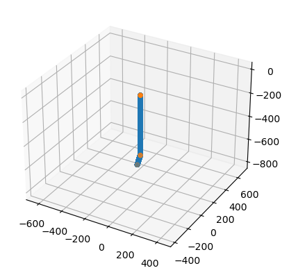
Interpolate/Resample between points

The second step is to resample linearly between each provided well path point. A spacing of 5 cm between each point is chosen by default.

points = gg.visualization.resample_between_well_deviation_points(coordinates)
pd.DataFrame(points, columns=['X', 'Y', 'Z'])

	X	Y	Z
0	0.000000	0.000000	0.000000
1	0.000000	0.000000	-0.050005
2	0.000000	0.000000	-0.100010
3	0.000000	0.000000	-0.150015
4	0.000000	0.000000	-0.200020
...	...	...	...
19376	-199.914712	299.872068	-799.872068
19377	-199.936034	299.904051	-799.904051
19378	-199.957356	299.936034	-799.936034
19379	-199.978678	299.968017	-799.968017
19380	-200.000000	300.000000	-800.000000

19381 rows × 3 columns

import matplotlib.pyplot as plt
fig = plt.figure()
ax = fig.add_subplot(projection='3d')
ax.scatter(points[:,0], points[:,1], points[:,2])
ax.scatter(coordinates[:,0], coordinates[:,1], coordinates[:,2])
ax.set_aspect('equal')
ax.grid()

Create Polyline from well path coordinates

Then, we create a polyline of the original well path for visualization purposes.

polyline_well_path = gg.visualization.polyline_from_points(coordinates)
polyline_well_path

PolyData	Information
N Cells	1
N Points	3
N Strips	0
X Bounds	-2.000e+02, 0.000e+00
Y Bounds	0.000e+00, 3.000e+02
Z Bounds	-8.000e+02, 0.000e+00
N Arrays	0

Creating Spline from resampled well path coordinates

Now, we are creating spline of the resampled points. This automatically calculates the arc_length which will be utilized in the next step.

polyline_well_path_resampled = pv.Spline(points)
polyline_well_path_resampled

Header	Data Arrays
PolyData Information N Cells 1 N Points 19381 N Strips 0 X Bounds -2.000e+02, 1.520e-03 Y Bounds -2.280e-03, 3.000e+02 Z Bounds -8.000e+02, 0.000e+00 N Arrays 1	Name Field Type N Comp Min Max arc_length Points float32 1 0.000e+00 9.690e+02

Getting the Points along the resampled Spline

The main step is to assign a resampled value to a measured value using get_points_along_spline.

points_along_spline = gg.visualization.get_points_along_spline(polyline_well_path_resampled, dist)
pd.DataFrame(points_along_spline, columns=['X', 'Y', 'Z'])

	X	Y	Z
0	0.000000	0.000000	0.000000
1	0.000000	0.000000	-1.000043
2	0.000000	0.000000	-2.000086
3	0.000000	0.000000	-3.000129
4	0.000000	0.000000	-4.000172
...	...	...	...
896	-168.850037	253.275055	-753.275085
897	-169.276459	253.914688	-753.914673
898	-169.702881	254.554321	-754.554321
899	-170.129303	255.193954	-755.193970
900	-170.555725	255.833572	-755.833557

901 rows × 3 columns

Creating Polyline from Points, assigning values and creating Tube

Once we have extracted the points, we again create a PolyLine from it. We then assign the measured well log values as data array to the newly created PolyLine and create a tube from it using the values to define the radius of the tube. The radius_factor is a scaling factor that needs to changed according to the length of the well.

polyline_along_spline = gg.visualization.polyline_from_points(points_along_spline)
polyline_along_spline['values'] = values
tube_along_spline = polyline_along_spline.tube(scalars='values', radius_factor=75)
tube_along_spline

Header	Data Arrays
PolyData Information N Cells 22 N Points 18060 N Strips 22 X Bounds -2.000e+02, 3.747e+01 Y Bounds -3.747e+01, 2.805e+02 Z Bounds -7.807e+02, 0.000e+00 N Arrays 2	Name Field Type N Comp Min Max values Points float64 1 3.398e-03 9.963e-01 TubeNormals Points float32 3 -9.992e-01 1.000e+00

Combined Function

tube_along_spline = show_well_log_along_well(coordinates, dist, values, radius_factor=75)
tube_along_spline

Header	Data Arrays
PolyData Information N Cells 22 N Points 18060 N Strips 22 X Bounds -2.000e+02, 3.747e+01 Y Bounds -3.747e+01, 2.805e+02 Z Bounds -7.807e+02, 0.000e+00 N Arrays 2	Name Field Type N Comp Min Max values Points float64 1 3.398e-03 9.963e-01 TubeNormals Points float32 3 -9.992e-01 1.000e+00

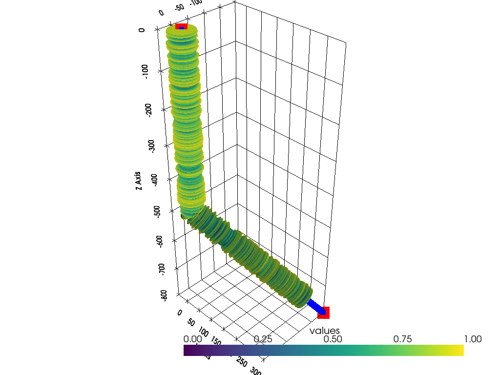
Plotting the result

sargs = dict(fmt="%.2f", color='black')

p = pv.Plotter(notebook=True)

p.add_mesh(tube_along_spline, scalar_bar_args=sargs, clim=[0,1])
p.add_mesh(pv.PolyData(coordinates), color='red', point_size=25)
p.add_mesh(pv.PolyData(points), color='blue', point_size=10)

p.set_background('white')
p.show_grid(color='black')
p.show()

C:\Users\ale93371\Anaconda3\envs\gempy_new8\lib\site-packages\pyvista\utilities\helpers.py:507: UserWarning: Points is not a float type. This can cause issues when transforming or applying filters. Casting to ``np.float32``. Disable this by passing ``force_float=False``.
  warnings.warn(
C:\Users\ale93371\Anaconda3\envs\gempy_new8\lib\site-packages\pyvista\jupyter\notebook.py:58: UserWarning: Failed to use notebook backend:

No module named 'trame'

Falling back to a static output.
  warnings.warn(