
Example 13 - Three Point Problem
Contents
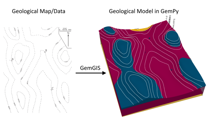
Example 13 - Three Point Problem#
This example will show how to convert the geological map below using GemGIS to a GemPy model. This example is based on digitized data. The area is 2991 m wide (W-E extent) and 3736 m high (N-S extent). The vertical model extent varies between 250 m and 1200 m. This example represents a classic “three-point-problem” of planar dippings layer (blue and purple) above an unspecified basement (yellow). The interface points were not taken at the surface but rather in boreholes
The map has been georeferenced with QGIS. The outcrops of the layers were digitized in QGIS. The contour lines were also digitized and will be interpolated with GemGIS to create a topography for the model.
Map Source: An Introduction to Geological Structures and Maps by G.M. Bennison
[1]:
import matplotlib.pyplot as plt
import matplotlib.image as mpimg
img = mpimg.imread('../images/cover_example13.png')
plt.figure(figsize=(10, 10))
imgplot = plt.imshow(img)
plt.axis('off')
plt.tight_layout()
Licensing#
Computational Geosciences and Reservoir Engineering, RWTH Aachen University, Authors: Alexander Juestel. For more information contact: alexander.juestel(at)rwth-aachen.de
This work is licensed under a Creative Commons Attribution 4.0 International License (http://creativecommons.org/licenses/by/4.0/)
Import GemGIS#
If you have installed GemGIS via pip or conda, you can import GemGIS like any other package. If you have downloaded the repository, append the path to the directory where the GemGIS repository is stored and then import GemGIS.
[2]:
import warnings
warnings.filterwarnings("ignore")
import gemgis as gg
Importing Libraries and loading Data#
All remaining packages can be loaded in order to prepare the data and to construct the model. The example data is downloaded from an external server using pooch. It will be stored in a data folder in the same directory where this notebook is stored.
[3]:
import geopandas as gpd
import rasterio
[4]:
file_path = 'data/example13/'
gg.download_gemgis_data.download_tutorial_data(filename="example13_three_point_problem.zip", dirpath=file_path)
Downloading file 'example13_three_point_problem.zip' from 'https://rwth-aachen.sciebo.de/s/AfXRsZywYDbUF34/download?path=%2Fexample13_three_point_problem.zip' to 'C:\Users\ale93371\Documents\gemgis\docs\getting_started\example\data\example13'.
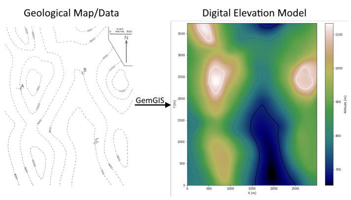
Creating Digital Elevation Model from Contour Lines#
The digital elevation model (DEM) will be created by interpolating contour lines digitized from the georeferenced map using the SciPy Radial Basis Function interpolation wrapped in GemGIS. The respective function used for that is gg.vector.interpolate_raster().
[5]:
import matplotlib.pyplot as plt
import matplotlib.image as mpimg
img = mpimg.imread('../images/dem_example13.png')
plt.figure(figsize=(10, 10))
imgplot = plt.imshow(img)
plt.axis('off')
plt.tight_layout()
[6]:
topo = gpd.read_file(file_path + 'topo13.shp')
topo.head()
[6]:
| id | Z | geometry | |
|---|---|---|---|
| 0 | None | 800 | LINESTRING (1.482 1748.098, 50.293 1669.250, 9... |
| 1 | None | 900 | LINESTRING (2.060 3333.723, 69.355 3237.834, 1... |
| 2 | None | 1000 | LINESTRING (681.366 917.450, 738.552 907.053, ... |
| 3 | None | 1000 | LINESTRING (36.141 3724.208, 57.225 3659.223, ... |
| 4 | None | 1100 | LINESTRING (249.868 3718.720, 252.467 3636.407... |
Interpolating the contour lines#
[7]:
topo_raster = gg.vector.interpolate_raster(gdf=topo, value='Z', method='rbf', res=10)
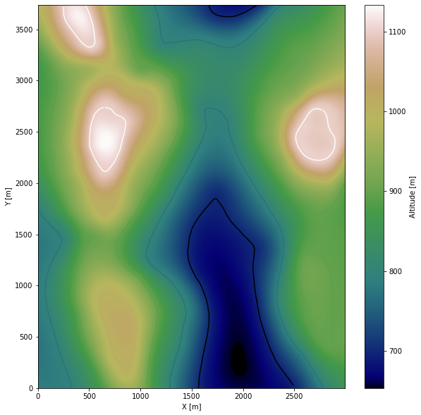
Plotting the raster#
[8]:
import matplotlib.pyplot as plt

fix, ax = plt.subplots(1, figsize=(10, 10))
topo.plot(ax=ax, aspect='equal', column='Z', cmap='gist_earth')
im = plt.imshow(topo_raster, origin='lower', extent=[0, 2991, 0, 3736], cmap='gist_earth')
cbar = plt.colorbar(im)
cbar.set_label('Altitude [m]')
ax.set_xlabel('X [m]')
ax.set_ylabel('Y [m]')
ax.set_xlim(0, 2991)
ax.set_ylim(0, 3736)
[8]:
(0.0, 3736.0)
Saving the raster to disc#
After the interpolation of the contour lines, the raster is saved to disc using gg.raster.save_as_tiff(). The function will not be executed as a raster is already provided with the example data.
Opening Raster#
The previously computed and saved raster can now be opened using rasterio.
[9]:
topo_raster = rasterio.open(file_path + 'raster13.tif')
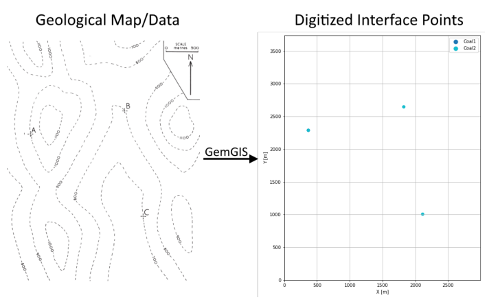
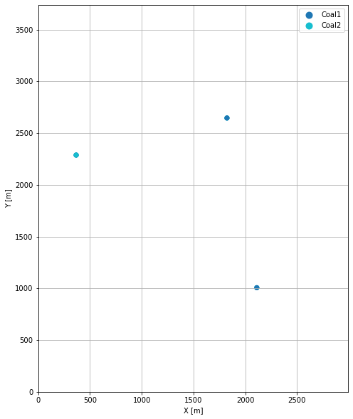
Interface Points of stratigraphic boundaries#
The interface points for this three point example will be digitized as points with the respective height value as given by the borehole information and the respective formation.
[10]:
import matplotlib.pyplot as plt
import matplotlib.image as mpimg
img = mpimg.imread('../images/interfaces_example13.png')
plt.figure(figsize=(10, 10))
imgplot = plt.imshow(img)
plt.axis('off')
plt.tight_layout()
[11]:
interfaces = gpd.read_file(file_path + 'interfaces13.shp')
interfaces.head()
[11]:
| id | formation | Z | geometry | |
|---|---|---|---|---|
| 0 | None | Coal1 | 950 | POINT (366.363 2287.350) |
| 1 | None | Coal2 | 550 | POINT (366.363 2287.350) |
| 2 | None | Coal2 | 650 | POINT (1822.758 2645.532) |
| 3 | None | Coal2 | 450 | POINT (2110.811 1006.118) |
| 4 | None | Coal1 | 1050 | POINT (1822.758 2645.532) |
Extracting Z coordinate from Digital Elevation Model#
[12]:
interfaces_coords = gg.vector.extract_xyz(gdf=interfaces, dem=None)
interfaces_coords
[12]:
| formation | Z | geometry | X | Y | |
|---|---|---|---|---|---|
| 0 | Coal1 | 950.00 | POINT (366.363 2287.350) | 366.36 | 2287.35 |
| 1 | Coal2 | 550.00 | POINT (366.363 2287.350) | 366.36 | 2287.35 |
| 2 | Coal2 | 650.00 | POINT (1822.758 2645.532) | 1822.76 | 2645.53 |
| 3 | Coal2 | 450.00 | POINT (2110.811 1006.118) | 2110.81 | 1006.12 |
| 4 | Coal1 | 1050.00 | POINT (1822.758 2645.532) | 1822.76 | 2645.53 |
| 5 | Coal1 | 850.00 | POINT (2110.811 1006.118) | 2110.81 | 1006.12 |
Plotting the Interface Points#
[13]:
fig, ax = plt.subplots(1, figsize=(10, 10))

interfaces.plot(ax=ax, column='formation', legend=True, aspect='equal')
interfaces_coords.plot(ax=ax, column='formation', legend=True, aspect='equal')
plt.grid()
ax.set_xlabel('X [m]')
ax.set_ylabel('Y [m]')
ax.set_xlim(0, 2991)
ax.set_ylim(0, 3736)
[13]:
(0.0, 3736.0)
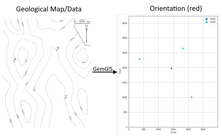
Orientations from Strike Lines#
For this three point example, an orientation is calculated using gg.vector.calculate_orientation_for_three_point_problem().
[14]:
import matplotlib.pyplot as plt
import matplotlib.image as mpimg
img = mpimg.imread('../images/orientations_example13.png')
plt.figure(figsize=(10, 10))
imgplot = plt.imshow(img)
plt.axis('off')
plt.tight_layout()
[15]:
import pandas as pd
orientations1 = gg.vector.calculate_orientation_for_three_point_problem(gdf=interfaces[interfaces['formation'] == 'Coal1'])
orientations2 = gg.vector.calculate_orientation_for_three_point_problem(gdf=interfaces[interfaces['formation'] == 'Coal2'])
orientations = pd.concat([orientations1, orientations2]).reset_index()
orientations
[15]:
| index | Z | formation | azimuth | dip | polarity | X | Y | geometry | |
|---|---|---|---|---|---|---|---|---|---|
| 0 | 0 | 950.0 | Coal1 | 16.09 | 172.38 | 1 | 1433.31 | 1979.67 | POINT (1433.311 1979.667) |
| 1 | 0 | 550.0 | Coal2 | 16.09 | 172.38 | 1 | 1433.31 | 1979.67 | POINT (1433.311 1979.667) |
Changing the Data Type of fields#
[16]:
orientations['Z'] = orientations['Z'].astype(float)
orientations['azimuth'] = orientations['azimuth'].astype(float)
orientations['dip'] = orientations['dip'].astype(float)
orientations['dip'] = 180 - orientations['dip']
orientations['azimuth'] = 180 - orientations['azimuth']
orientations['polarity'] = orientations['polarity'].astype(float)
orientations['X'] = orientations['X'].astype(float)
orientations['Y'] = orientations['Y'].astype(float)
orientations.info()
<class 'geopandas.geodataframe.GeoDataFrame'>
RangeIndex: 2 entries, 0 to 1
Data columns (total 9 columns):
 #   Column     Non-Null Count  Dtype
---  ------     --------------  -----
 0   index      2 non-null      int64
 1   Z          2 non-null      float64
 2   formation  2 non-null      object
 3   azimuth    2 non-null      float64
 4   dip        2 non-null      float64
 5   polarity   2 non-null      float64
 6   X          2 non-null      float64
 7   Y          2 non-null      float64
 8   geometry   2 non-null      geometry
dtypes: float64(6), geometry(1), int64(1), object(1)
memory usage: 272.0+ bytes
[17]:
orientations
[17]:
| index | Z | formation | azimuth | dip | polarity | X | Y | geometry | |
|---|---|---|---|---|---|---|---|---|---|
| 0 | 0 | 950.00 | Coal1 | 163.91 | 7.62 | 1.00 | 1433.31 | 1979.67 | POINT (1433.311 1979.667) |
| 1 | 0 | 550.00 | Coal2 | 163.91 | 7.62 | 1.00 | 1433.31 | 1979.67 | POINT (1433.311 1979.667) |
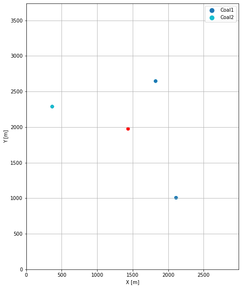
Plotting the Orientations#
[18]:
fig, ax = plt.subplots(1, figsize=(10, 10))

interfaces.plot(ax=ax, column='formation', legend=True, aspect='equal')
interfaces_coords.plot(ax=ax, column='formation', legend=True, aspect='equal')
orientations.plot(ax=ax, color='red', aspect='equal')
plt.grid()
ax.set_xlabel('X [m]')
ax.set_ylabel('Y [m]')
ax.set_xlim(0, 2991)
ax.set_ylim(0, 3736)
[18]:
(0.0, 3736.0)
GemPy Model Construction#
The structural geological model will be constructed using the GemPy package.
[19]:
import gempy as gp
WARNING (theano.configdefaults): g++ not available, if using conda: `conda install m2w64-toolchain`
WARNING (theano.configdefaults): g++ not detected ! Theano will be unable to execute optimized C-implementations (for both CPU and GPU) and will default to Python implementations. Performance will be severely degraded. To remove this warning, set Theano flags cxx to an empty string.
WARNING (theano.tensor.blas): Using NumPy C-API based implementation for BLAS functions.
Creating new Model#
[20]:
geo_model = gp.create_model('Model13')
geo_model
[20]:
Model13 2022-04-05 11:05
Initiate Data#
[21]:
gp.init_data(geo_model, [0, 2991, 0, 3736, 250, 1200], [100, 100, 100],
             surface_points_df=interfaces_coords[interfaces_coords['Z'] != 0],
             orientations_df=orientations,
             default_values=True)
Active grids: ['regular']
[21]:
Model13 2022-04-05 11:05
Model Surfaces#
[22]:
geo_model.surfaces
[22]:
| surface | series | order_surfaces | color | id | |
|---|---|---|---|---|---|
| 0 | Coal1 | Default series | 1 | #015482 | 1 |
| 1 | Coal2 | Default series | 2 | #9f0052 | 2 |
Mapping the Stack to Surfaces#
[23]:
gp.map_stack_to_surfaces(geo_model,
                         {
                          'Strata1': ('Coal1', 'Coal2'),
                         },
                         remove_unused_series=True)
geo_model.add_surfaces('Basement')
[23]:
| surface | series | order_surfaces | color | id | |
|---|---|---|---|---|---|
| 0 | Coal1 | Strata1 | 1 | #015482 | 1 |
| 1 | Coal2 | Strata1 | 2 | #9f0052 | 2 |
| 2 | Basement | Strata1 | 3 | #ffbe00 | 3 |
Showing the Number of Data Points#
[24]:
gg.utils.show_number_of_data_points(geo_model=geo_model)
[24]:
| surface | series | order_surfaces | color | id | No. of Interfaces | No. of Orientations | |
|---|---|---|---|---|---|---|---|
| 0 | Coal1 | Strata1 | 1 | #015482 | 1 | 3 | 1 |
| 1 | Coal2 | Strata1 | 2 | #9f0052 | 2 | 3 | 1 |
| 2 | Basement | Strata1 | 3 | #ffbe00 | 3 | 0 | 0 |
Loading Digital Elevation Model#
[25]:
geo_model.set_topography(
    source='gdal', filepath=file_path + 'raster13.tif')
Cropped raster to geo_model.grid.extent.
depending on the size of the raster, this can take a while...
storing converted file...
Active grids: ['regular' 'topography']
[25]:
Grid Object. Values:
array([[  14.955     ,   18.68      ,  254.75      ],
       [  14.955     ,   18.68      ,  264.25      ],
       [  14.955     ,   18.68      ,  273.75      ],
       ...,
       [2985.99832776, 3711.02673797,  907.33477783],
       [2985.99832776, 3721.01604278,  906.7131958 ],
       [2985.99832776, 3731.00534759,  906.11096191]])
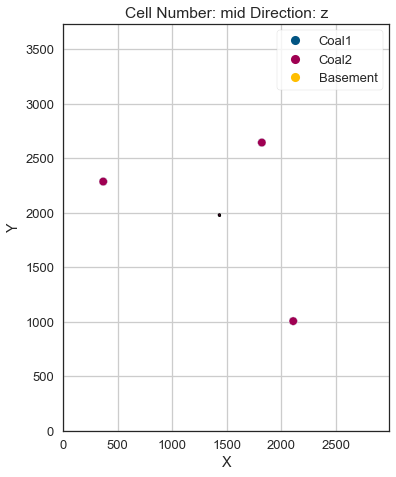
Plotting Input Data#
[26]:
gp.plot_2d(geo_model, direction='z', show_lith=False, show_boundaries=False)
plt.grid()
[27]:
gp.plot_3d(geo_model, image=False, plotter_type='basic', notebook=True)
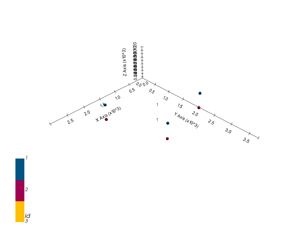
[27]:
<gempy.plot.vista.GemPyToVista at 0x1f20d692d30>
Setting the Interpolator#
[28]:
gp.set_interpolator(geo_model,
                    compile_theano=True,
                    theano_optimizer='fast_compile',
                    verbose=[],
                    update_kriging=False
                    )
Compiling theano function...
Level of Optimization:  fast_compile
Device:  cpu
Precision:  float64
Number of faults:  0
Compilation Done!
Kriging values:
                    values
range             4879.17
$C_o$           566816.12
drift equations       [3]
[28]:
<gempy.core.interpolator.InterpolatorModel at 0x1f205cb0970>
Computing Model#
[29]:
sol = gp.compute_model(geo_model, compute_mesh=True)
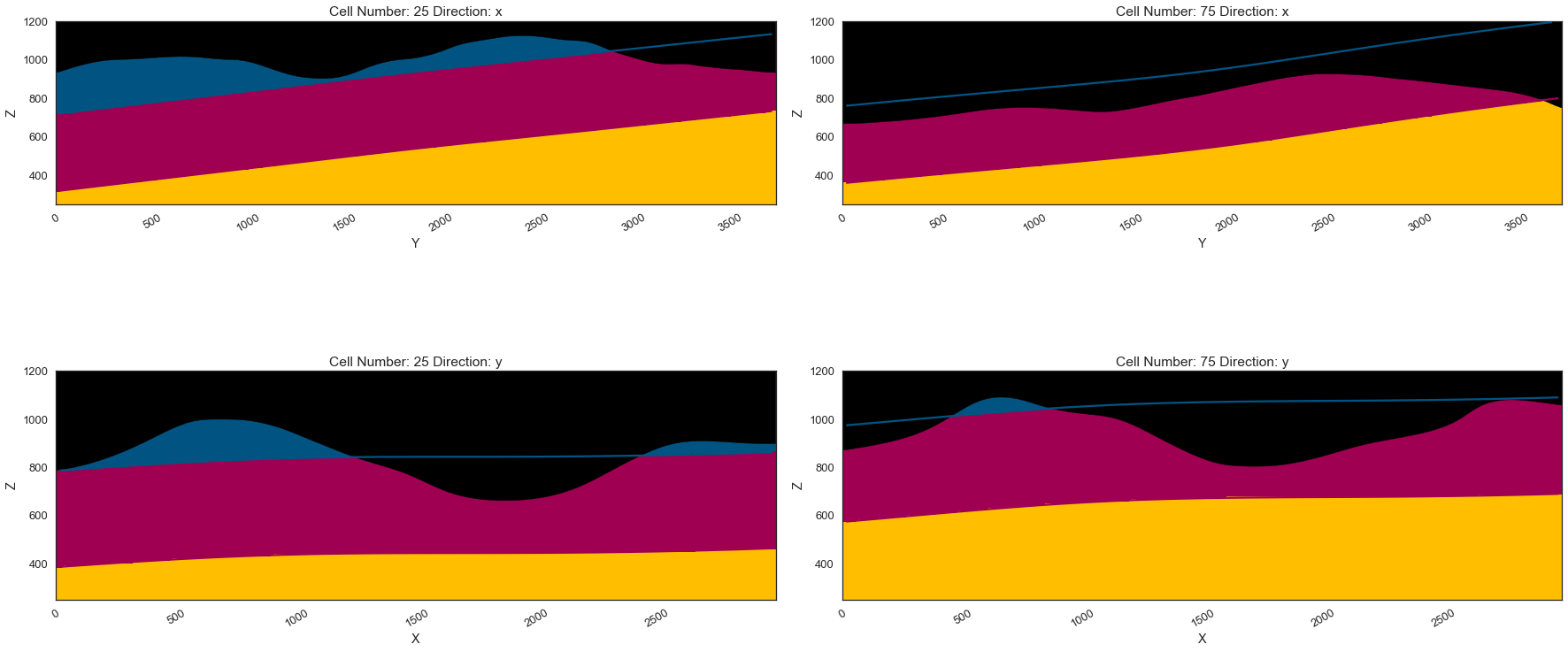
Plotting Cross Sections#
[30]:
gp.plot_2d(geo_model, direction=['x', 'x', 'y', 'y'], cell_number=[25, 75, 25, 75], show_topography=True, show_data=False)
[30]:
<gempy.plot.visualization_2d.Plot2D at 0x1f212ac02e0>
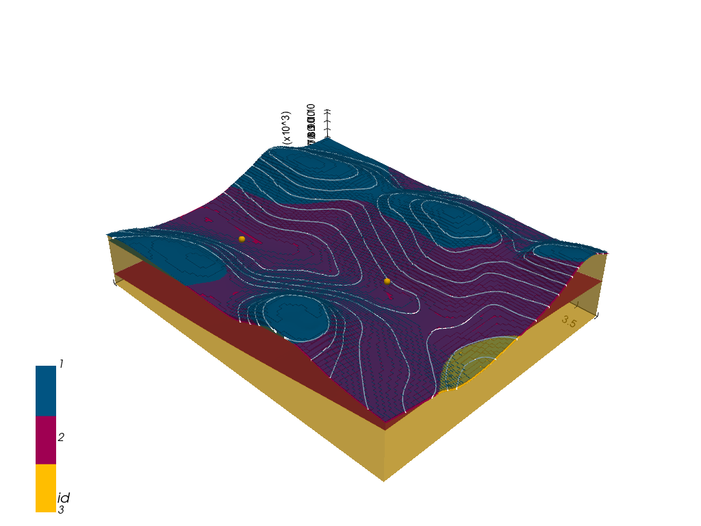
Plotting 3D Model#
[31]:
gpv = gp.plot_3d(geo_model, image=False, show_topography=True,
                 plotter_type='basic', notebook=True, show_lith=True)
[ ]: