68 Creating Finite Faults with GemGIS
Contents
68 Creating Finite Faults with GemGIS#
This notebook illustrates how to create finite faults from a GemPy Model. Here, we will use an elongated version of the Graben Model to later create the finite faults.
Set File Paths and download Tutorial Data#
If you downloaded the latest GemGIS version from the Github repository, append the path so that the package can be imported successfully. Otherwise, it is recommended to install GemGIS via pip install gemgis and import GemGIS using import gemgis as gg. In addition, the file path to the folder where the data is being stored is set. The tutorial data is downloaded using Pooch (https://www.fatiando.org/pooch/latest/index.html) and stored in the specified folder. Use
pip install pooch if Pooch is not installed on your system yet.
[1]:
import warnings
warnings.filterwarnings("ignore")

import gempy as gp
import gemgis as gg
import pandas as pd
import geopandas as gpd

import pyvista as pv
WARNING (aesara.configdefaults): g++ not available, if using conda: `conda install m2w64-toolchain`
WARNING (aesara.configdefaults): g++ not detected!  Aesara will be unable to compile C-implementations and will default to Python. Performance may be severely degraded. To remove this warning, set Aesara flags cxx to an empty string.
WARNING (aesara.tensor.blas): Using NumPy C-API based implementation for BLAS functions.
[2]:
file_path ='data/68_Creating_Finite_Faults_with_GemGIS/'
# gg.download_gemgis_data.download_tutorial_data(filename="68_creating_finite_faults_with_gemgis.zip", dirpath=file_path)
Loading Input Data#
[3]:
interfaces = pd.read_csv(file_path + 'interfaces.csv', delimiter=';')
interfaces.head()
[3]:
| X | Y | Z | formation | |
|---|---|---|---|---|
| 0 | 200 | 250 | -100 | Layer1 |
| 1 | 200 | 500 | -100 | Layer1 |
| 2 | 200 | 750 | -100 | Layer1 |
| 3 | 200 | 250 | -200 | Layer2 |
| 4 | 200 | 500 | -200 | Layer2 |
[4]:
orientations = pd.read_csv(file_path + 'orientations.csv', delimiter=';')
orientations.head()
[4]:
| X | Y | Z | formation | dip | azimuth | polarity | |
|---|---|---|---|---|---|---|---|
| 0 | 200 | 500 | -100 | Layer1 | 0 | 0 | 1 |
| 1 | 800 | 500 | -100 | Layer1 | 0 | 0 | 1 |
| 2 | 500 | 500 | -300 | Layer1 | 0 | 0 | 1 |
| 3 | 250 | 500 | -100 | Fault1 | 60 | 90 | 1 |
| 4 | 750 | 500 | -100 | Fault2 | 60 | 270 | 1 |
Creating the GemPy Model#
[5]:
geo_model = gp.create_model('Graben_Model')
geo_model
[5]:
Graben_Model 2023-10-10 16:03
[6]:
gp.init_data(geo_model, [0, 1000, -500, 1500, -600, 0], [50,50,50],
             surface_points_df=interfaces,
             orientations_df=orientations,
             default_values=True)

gp.map_stack_to_surfaces(geo_model,
                         {
                          'Fault1': ('Fault1'),
                          'Fault2': ('Fault2'),
                          'Strata1': ('Layer1', 'Layer2', 'Layer3'),
                         },
                         remove_unused_series=True)
geo_model.add_surfaces('Basement')
geo_model.set_is_fault(['Fault1', 'Fault2'])
geo_model.set_topography(source='random')
gp.set_interpolator(geo_model,
                    compile_theano=True,
                    theano_optimizer='fast_compile',
                    verbose=[],
                    update_kriging=False
                    )
geo_model.surfaces
Active grids: ['regular']
Fault colors changed. If you do not like this behavior, set change_color to False.
Fault colors changed. If you do not like this behavior, set change_color to False.
[-120.    0.]
Active grids: ['regular' 'topography']
Compiling aesara function...
Level of Optimization:  fast_compile
Device:  cpu
Precision:  float64
Number of faults:  2
Compilation Done!
Kriging values:
                     values
range              2315.17
$C_o$            127619.05
drift equations  [3, 3, 3]
[6]:
| surface | series | order_surfaces | color | id | |
|---|---|---|---|---|---|
| 3 | Fault1 | Fault1 | 1 | #527682 | 1 |
| 4 | Fault2 | Fault2 | 1 | #527682 | 2 |
| 0 | Layer1 | Strata1 | 1 | #ffbe00 | 3 |
| 1 | Layer2 | Strata1 | 2 | #728f02 | 4 |
| 2 | Layer3 | Strata1 | 3 | #443988 | 5 |
| 5 | Basement | Strata1 | 4 | #ff3f20 | 6 |
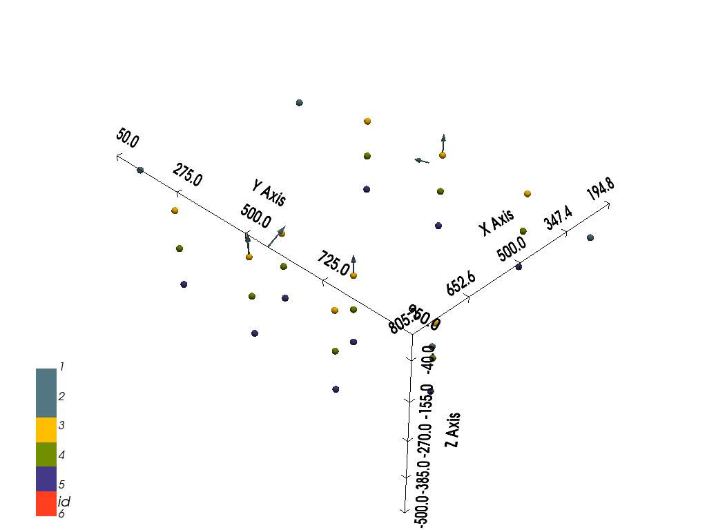
[7]:
gp.plot_3d(geo_model, image=False, plotter_type='basic', notebook=True)
[7]:
<gempy.plot.vista.GemPyToVista at 0x25557e1ba90>
[8]:
sol = gp.compute_model(geo_model, compute_mesh=True)
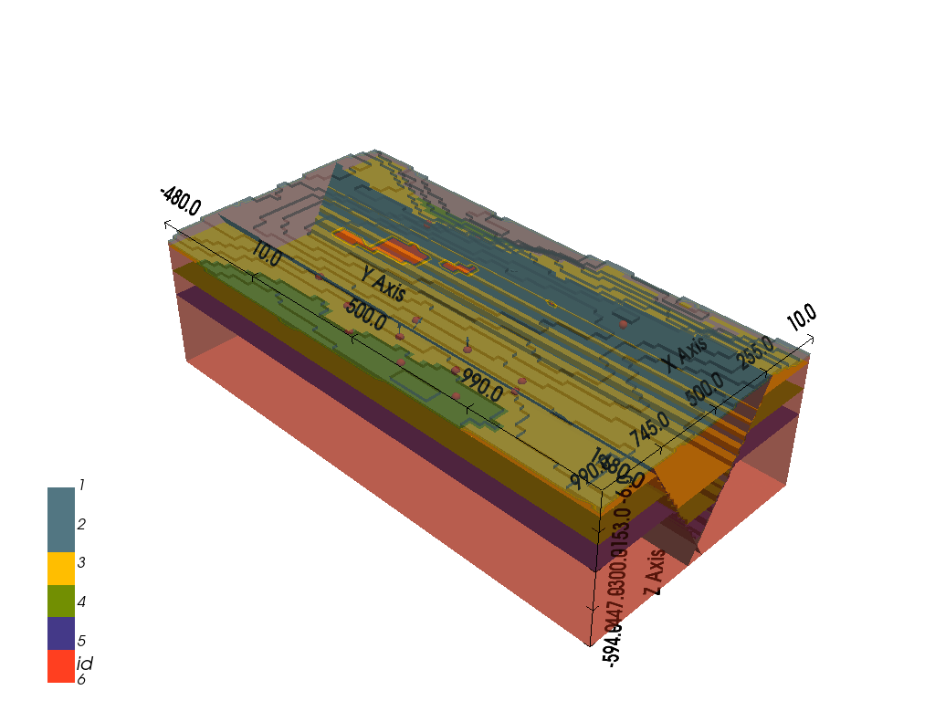
[9]:
gp.plot_3d(geo_model, notebook=True)
[9]:
<gempy.plot.vista.GemPyToVista at 0x2555b0d0340>
Creating Finite Faults from GemPy Model#
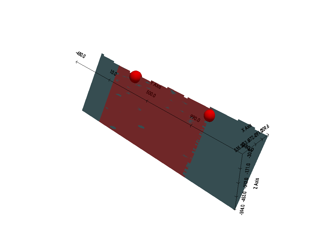
Finite faults will be created during a postprocessing step performed in GemGIS. Here, we are using the function clip_fault_of_gempy_model(..) to clip a fault. By default, the fault will be clipped at the first or last interface point (both sides can be chosen). In addition, a buffer along the strike of the fault can be chosen to allow the fault to extend beyond the last interface point if wished.
Here, we are choosing to clip the fault on both ends. For the one end, we would like to have a 250 m buffer so that the fault extends beyond the first point. For the last point, we do not want to have a buffer.
[10]:
mesh = gg.postprocessing.clip_fault_of_gempy_model(geo_model,fault='Fault1',
                                                   which='both',
                                                   buffer_first=250,
                                                   buffer_last=0)
mesh
[10]:
{'Fault1': [PolyData (0x2555e8d5300)
    N Cells:    3512
    N Points:   1881
    N Strips:   0
    X Bounds:   2.165e+02, 5.352e+02
    Y Bounds:   -2.000e+02, 9.500e+02
    Z Bounds:   -5.940e+02, -4.200e+01
    N Arrays:   1,
  '#527682']}
[11]:
fault_polydata = pv.PolyData(interfaces[interfaces['formation']=='Fault1'][['X', 'Y', 'Z']].values)
fault_polydata
[11]:
| PolyData | Information |
|---|---|
| N Cells | 2 |
| N Points | 2 |
| N Strips | 0 |
| X Bounds | 2.500e+02, 2.500e+02 |
| Y Bounds | 5.000e+01, 9.500e+02 |
| Z Bounds | -1.000e+02, -1.000e+02 |
| N Arrays | 0 |
[12]:
mesh1 = gg.visualization.create_depth_maps_from_gempy(geo_model, surfaces='Fault1')
mesh1
[12]:
{'Fault1': [PolyData (0x2556ca0b5e0)
    N Cells:    5902
    N Points:   3070
    N Strips:   0
    X Bounds:   2.096e+02, 5.352e+02
    Y Bounds:   -4.800e+02, 1.480e+03
    Z Bounds:   -5.940e+02, -3.000e+01
    N Arrays:   1,
  '#527682']}
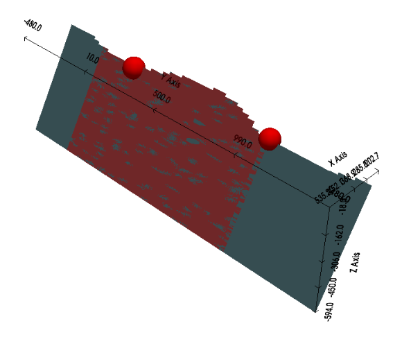
Plotting the Result#
Plotting the result, we can see the interface points of the fault (red spheres), the original extent of the fault modeled by GemPy in gray and the clipped fault (finite fault) with a buffer on one side in red.
[13]:
p = pv.Plotter(notebook=True)

p.add_mesh(mesh['Fault1'][0], color='red', opacity=0.5)
p.add_mesh(mesh1['Fault1'][0], color=mesh1['Fault1'][1])

p.add_mesh(fault_polydata, color='red', point_size=40, render_points_as_spheres=True)

p.set_background('white')
p.set_scale(1,1,1)
p.show_bounds(color='black', font_size=12)

p.show()