
Example 17 - Three Point Problem and Folded Layers
Contents
Example 17 - Three Point Problem and Folded Layers#
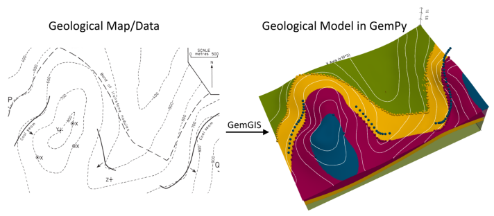
This example will show how to convert the geological map below using GemGIS to a GemPy model. This example is based on digitized data. The area is 3892 m wide (W-E extent) and 2683 m high (N-S extent). The model represents a coal seam that was encountered at the surface and in boreholes. A second coal seam is located 300 m vertically above the first one. The vertical model extent varies between 0 m and 1000 m.
The map has been georeferenced with QGIS. The stratigraphic boundaries were digitized in QGIS. Strikes lines were digitized in QGIS as well and will be used to calculate orientations for the GemPy model. The contour lines were also digitized and will be interpolated with GemGIS to create a topography for the model.
Map Source: An Introduction to Geological Structures and Maps by G.M. Bennison
[1]:
import matplotlib.pyplot as plt
import matplotlib.image as mpimg
img = mpimg.imread('../images/cover_example17.png')
plt.figure(figsize=(10, 10))
imgplot = plt.imshow(img)
plt.axis('off')
plt.tight_layout()
Licensing#
Computational Geosciences and Reservoir Engineering, RWTH Aachen University, Authors: Alexander Juestel. For more information contact: alexander.juestel(at)rwth-aachen.de
This work is licensed under a Creative Commons Attribution 4.0 International License (http://creativecommons.org/licenses/by/4.0/)
Import GemGIS#
If you have installed GemGIS via pip or conda, you can import GemGIS like any other package. If you have downloaded the repository, append the path to the directory where the GemGIS repository is stored and then import GemGIS.
[2]:
import warnings
warnings.filterwarnings("ignore")
import gemgis as gg
Importing Libraries and loading Data#
All remaining packages can be loaded in order to prepare the data and to construct the model. The example data is downloaded from an external server using pooch. It will be stored in a data folder in the same directory where this notebook is stored.
[3]:
import geopandas as gpd
import rasterio
[4]:
file_path = 'data/example17/'
gg.download_gemgis_data.download_tutorial_data(filename="example17_three_point_problem.zip", dirpath=file_path)
Downloading file 'example17_three_point_problem.zip' from 'https://rwth-aachen.sciebo.de/s/AfXRsZywYDbUF34/download?path=%2Fexample17_three_point_problem.zip' to 'C:\Users\ale93371\Documents\gemgis\docs\getting_started\example\data\example17'.
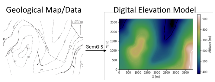
Creating Digital Elevation Model from Contour Lines#
The digital elevation model (DEM) will be created by interpolating contour lines digitized from the georeferenced map using the SciPy Radial Basis Function interpolation wrapped in GemGIS. The respective function used for that is gg.vector.interpolate_raster().
[5]:
import matplotlib.pyplot as plt
import matplotlib.image as mpimg
img = mpimg.imread('../images/dem_example17.png')
plt.figure(figsize=(10, 10))
imgplot = plt.imshow(img)
plt.axis('off')
plt.tight_layout()
[6]:
topo = gpd.read_file(file_path + 'topo17.shp')
topo.head()
[6]:
| id | Z | geometry | |
|---|---|---|---|
| 0 | None | 600 | LINESTRING (399.582 9.701, 373.041 104.254, 35... |
| 1 | None | 900 | LINESTRING (3680.737 2.651, 3702.716 47.854, 3... |
| 2 | None | 800 | LINESTRING (3390.857 3.480, 3398.322 17.995, 3... |
| 3 | None | 700 | LINESTRING (2564.763 4.725, 2631.530 33.339, 2... |
| 4 | None | 800 | LINESTRING (1224.018 1463.246, 1211.577 1384.4... |
Interpolating the contour lines#
[7]:
topo_raster = gg.vector.interpolate_raster(gdf=topo, value='Z', method='rbf', res=10)
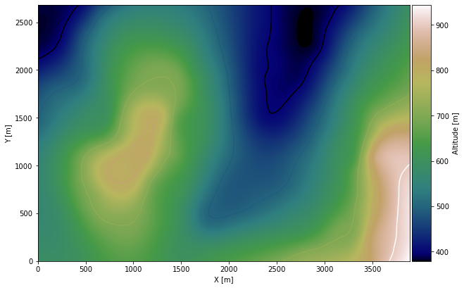
Plotting the raster#
[8]:
import matplotlib.pyplot as plt

from mpl_toolkits.axes_grid1 import make_axes_locatable

fix, ax = plt.subplots(1, figsize=(10, 10))
topo.plot(ax=ax, aspect='equal', column='Z', cmap='gist_earth')
im = plt.imshow(topo_raster, origin='lower', extent=[0, 3892, 0, 2683], cmap='gist_earth')
divider = make_axes_locatable(ax)
cax = divider.append_axes("right", size="5%", pad=0.05)
cbar = plt.colorbar(im, cax=cax)
cbar.set_label('Altitude [m]')
ax.set_xlabel('X [m]')
ax.set_ylabel('Y [m]')
ax.set_xlim(0, 3892)
ax.set_ylim(0, 2683)
[8]:
(0.0, 2683.0)
Saving the raster to disc#
After the interpolation of the contour lines, the raster is saved to disc using gg.raster.save_as_tiff(). The function will not be executed as a raster is already provided with the example data.
Opening Raster#
The previously computed and saved raster can now be opened using rasterio.
[9]:
topo_raster = rasterio.open(file_path + 'raster17.tif')
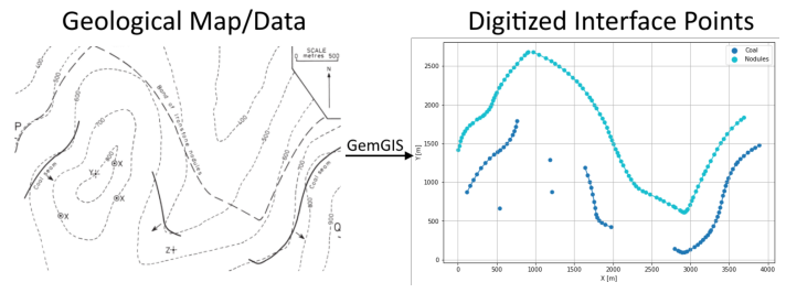
Interface Points of stratigraphic boundaries#
The interface points will be extracted from LineStrings digitized from the georeferenced map using QGIS. It is important to provide a formation name for each layer boundary. The vertical position of the interface point will be extracted from the digital elevation model using the GemGIS function gg.vector.extract_xyz(). The resulting GeoDataFrame now contains single points including the information about the respective formation.
[10]:
import matplotlib.pyplot as plt
import matplotlib.image as mpimg
img = mpimg.imread('../images/interfaces_example17.png')
plt.figure(figsize=(10, 10))
imgplot = plt.imshow(img)
plt.axis('off')
plt.tight_layout()
[11]:
interfaces = gpd.read_file(file_path + 'interfaces17.shp')
interfaces.head()
[11]:
| id | formation | geometry | |
|---|---|---|---|
| 0 | None | Coal | LINESTRING (117.997 870.009, 159.675 952.743, ... |
| 1 | None | Nodules | LINESTRING (4.782 1414.932, 21.578 1466.563, 3... |
| 2 | None | Nodules | LINESTRING (974.572 2678.334, 1047.353 2644.74... |
| 3 | None | Coal | LINESTRING (1643.286 1185.393, 1675.011 1087.1... |
| 4 | None | Coal | LINESTRING (2798.761 137.845, 2842.927 113.585... |
Extracting Z coordinate from Digital Elevation Model#
[12]:
interfaces_coords = gg.vector.extract_xyz(gdf=interfaces, dem=topo_raster)
interfaces_coords = interfaces_coords.sort_values(by='formation', ascending=True)
interfaces_coords.head()
[12]:
| formation | geometry | X | Y | Z | |
|---|---|---|---|---|---|
| 0 | Coal | POINT (117.997 870.009) | 118.00 | 870.01 | 583.24 |
| 141 | Coal | POINT (3095.794 190.409) | 3095.79 | 190.41 | 703.05 |
| 140 | Coal | POINT (3054.116 161.483) | 3054.12 | 161.48 | 705.77 |
| 139 | Coal | POINT (2999.064 127.892) | 2999.06 | 127.89 | 708.86 |
| 138 | Coal | POINT (2956.764 103.010) | 2956.76 | 103.01 | 710.91 |
[13]:
points = gpd.read_file(file_path + 'points17.shp')
points
[13]:
| id | formation | Z | geometry | |
|---|---|---|---|---|
| 0 | None | Coal | 500 | POINT (1191.049 1286.166) |
| 1 | None | Coal | 400 | POINT (1215.931 871.875) |
| 2 | None | Coal | 400 | POINT (541.619 659.753) |
[14]:
points_coords = gg.vector.extract_xy(gdf=points)
points_coords
[14]:
| formation | Z | geometry | X | Y | |
|---|---|---|---|---|---|
| 0 | Coal | 500.00 | POINT (1191.049 1286.166) | 1191.05 | 1286.17 |
| 1 | Coal | 400.00 | POINT (1215.931 871.875) | 1215.93 | 871.87 |
| 2 | Coal | 400.00 | POINT (541.619 659.753) | 541.62 | 659.75 |
[15]:
import pandas as pd

interfaces_coords = pd.concat([interfaces_coords, points_coords])
interfaces_coords = interfaces_coords[interfaces_coords['formation'].isin(['Coal', 'Nodules'])].reset_index()
interfaces_coords.head()
[15]:
| index | formation | geometry | X | Y | Z | |
|---|---|---|---|---|---|---|
| 0 | 0 | Coal | POINT (117.997 870.009) | 118.00 | 870.01 | 583.24 |
| 1 | 141 | Coal | POINT (3095.794 190.409) | 3095.79 | 190.41 | 703.05 |
| 2 | 140 | Coal | POINT (3054.116 161.483) | 3054.12 | 161.48 | 705.77 |
| 3 | 139 | Coal | POINT (2999.064 127.892) | 2999.06 | 127.89 | 708.86 |
| 4 | 138 | Coal | POINT (2956.764 103.010) | 2956.76 | 103.01 | 710.91 |
Creating data for the coal seam 300 m heigher#
[16]:
interfaces_coal300 = interfaces_coords[interfaces_coords['formation']=='Coal']
interfaces_coal300['Z'] = interfaces_coal300['Z']+300
interfaces_coal300['formation'] = 'Coal300'
interfaces_coal300
[16]:
| index | formation | geometry | X | Y | Z | |
|---|---|---|---|---|---|---|
| 0 | 0 | Coal300 | POINT (117.997 870.009) | 118.00 | 870.01 | 883.24 |
| 1 | 141 | Coal300 | POINT (3095.794 190.409) | 3095.79 | 190.41 | 1003.05 |
| 2 | 140 | Coal300 | POINT (3054.116 161.483) | 3054.12 | 161.48 | 1005.77 |
| 3 | 139 | Coal300 | POINT (2999.064 127.892) | 2999.06 | 127.89 | 1008.86 |
| 4 | 138 | Coal300 | POINT (2956.764 103.010) | 2956.76 | 103.01 | 1010.91 |
| ... | ... | ... | ... | ... | ... | ... |
| 64 | 1 | Coal300 | POINT (159.675 952.743) | 159.68 | 952.74 | 892.40 |
| 65 | 7 | Coal300 | POINT (468.216 1355.837) | 468.22 | 1355.84 | 906.89 |
| 169 | 0 | Coal300 | POINT (1191.049 1286.166) | 1191.05 | 1286.17 | 800.00 |
| 170 | 1 | Coal300 | POINT (1215.931 871.875) | 1215.93 | 871.87 | 700.00 |
| 171 | 2 | Coal300 | POINT (541.619 659.753) | 541.62 | 659.75 | 700.00 |
69 rows × 6 columns
Merging the interface data#
[17]:
interfaces_coords = pd.concat([interfaces_coal300, interfaces_coords])
interfaces_coords = interfaces_coords[interfaces_coords['formation'].isin(['Coal300', 'Coal', 'Nodules'])].reset_index()
interfaces_coords.head()
[17]:
| level_0 | index | formation | geometry | X | Y | Z | |
|---|---|---|---|---|---|---|---|
| 0 | 0 | 0 | Coal300 | POINT (117.997 870.009) | 118.00 | 870.01 | 883.24 |
| 1 | 1 | 141 | Coal300 | POINT (3095.794 190.409) | 3095.79 | 190.41 | 1003.05 |
| 2 | 2 | 140 | Coal300 | POINT (3054.116 161.483) | 3054.12 | 161.48 | 1005.77 |
| 3 | 3 | 139 | Coal300 | POINT (2999.064 127.892) | 2999.06 | 127.89 | 1008.86 |
| 4 | 4 | 138 | Coal300 | POINT (2956.764 103.010) | 2956.76 | 103.01 | 1010.91 |
Plotting the Interface Points#
[18]:
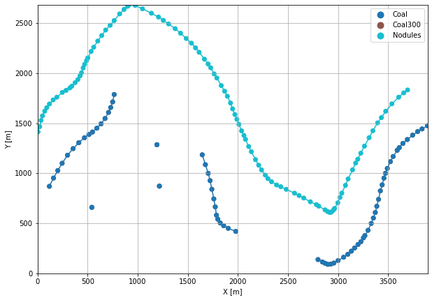
fig, ax = plt.subplots(1, figsize=(10, 10))

interfaces.plot(ax=ax, column='formation', legend=True, aspect='equal')
interfaces_coords.plot(ax=ax, column='formation', legend=True, aspect='equal')
points_coords.plot(ax=ax, column='formation', legend=False, aspect='equal')
plt.grid()
ax.set_xlabel('X [m]')
ax.set_ylabel('Y [m]')
ax.set_xlim(0, 3892)
ax.set_ylim(0, 2683)
[18]:
(0.0, 2683.0)
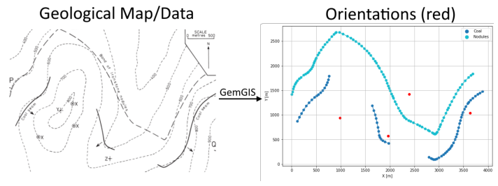
Orientations from Strike Lines#
Strike lines connect outcropping stratigraphic boundaries (interfaces) of the same altitude. In other words: the intersections between topographic contours and stratigraphic boundaries at the surface. The height difference and the horizontal difference between two digitized lines is used to calculate the dip and azimuth and hence an orientation that is necessary for GemPy. In order to calculate the orientations, each set of strikes lines/LineStrings for one formation must be given an id
number next to the altitude of the strike line. The id field is already predefined in QGIS. The strike line with the lowest altitude gets the id number 1, the strike line with the highest altitude the the number according to the number of digitized strike lines. It is currently recommended to use one set of strike lines for each structural element of one formation as illustrated.
[19]:
import matplotlib.pyplot as plt
import matplotlib.image as mpimg
img = mpimg.imread('../images/orientations_example17.png')
plt.figure(figsize=(10, 10))
imgplot = plt.imshow(img)
plt.axis('off')
plt.tight_layout()
[20]:
strikes = gpd.read_file(file_path + 'strikes17.shp')
strikes.head()
[20]:
| id | formation | Z | geometry | |
|---|---|---|---|---|
| 0 | 2 | Coal2 | 800 | LINESTRING (3799.965 1421.775, 3474.006 1008.728) |
| 1 | 1 | Coal2 | 700 | LINESTRING (3158.000 249.816, 4109.750 1469.052) |
| 2 | 1 | Coal1 | 500 | LINESTRING (1793.202 564.267, 1911.393 443.898) |
| 3 | 2 | Coal1 | 600 | LINESTRING (1667.546 1093.328, 2477.467 175.791) |
| 4 | 1 | Nodules | 500 | LINESTRING (2038.915 1418.665, 2585.083 789.763) |
Calculate Orientations for each formation#
[21]:
orientations_coal1 = gg.vector.calculate_orientations_from_strike_lines(gdf=strikes[strikes['formation'] == 'Coal1'].sort_values(by='Z', ascending=True).reset_index())
orientations_coal1
[21]:
| dip | azimuth | Z | geometry | polarity | formation | X | Y | |
|---|---|---|---|---|---|---|---|---|
| 0 | 22.04 | 228.51 | 550.00 | POINT (1962.402 569.321) | 1.00 | Coal1 | 1962.40 | 569.32 |
[22]:
orientations_coal2 = gg.vector.calculate_orientations_from_strike_lines(gdf=strikes[strikes['formation'] == 'Coal2'].sort_values(by='Z', ascending=True).reset_index())
orientations_coal2
[22]:
| dip | azimuth | Z | geometry | polarity | formation | X | Y | |
|---|---|---|---|---|---|---|---|---|
| 0 | 24.93 | 128.01 | 750.00 | POINT (3635.430 1037.343) | 1.00 | Coal2 | 3635.43 | 1037.34 |
[23]:
orientations_nodules = gg.vector.calculate_orientations_from_strike_lines(gdf=strikes[strikes['formation'] == 'Nodules'].sort_values(by='Z', ascending=True).reset_index())
orientations_nodules
[23]:
| dip | azimuth | Z | geometry | polarity | formation | X | Y | |
|---|---|---|---|---|---|---|---|---|
| 0 | 10.45 | 228.04 | 550.00 | POINT (2395.977 1421.931) | 1.00 | Nodules | 2395.98 | 1421.93 |
[24]:
orientations_coal3 = gg.vector.calculate_orientation_for_three_point_problem(gdf=points)
orientations_coal3['Z'] = orientations_coal3['Z'].astype(float)
orientations_coal3['azimuth'] = orientations_coal3['azimuth'].astype(float)
orientations_coal3['dip'] = orientations_coal3['dip'].astype(float)
orientations_coal3['dip'] = 180 - orientations_coal3['dip']
orientations_coal3['azimuth'] = 180 - orientations_coal3['azimuth']
orientations_coal3['polarity'] = orientations_coal3['polarity'].astype(float)
orientations_coal3['X'] = orientations_coal3['X'].astype(float)
orientations_coal3['Y'] = orientations_coal3['Y'].astype(float)
orientations_coal3
[24]:
| Z | formation | azimuth | dip | polarity | X | Y | geometry | |
|---|---|---|---|---|---|---|---|---|
| 0 | 433.33 | Coal | 197.46 | 13.95 | 1.00 | 982.87 | 939.26 | POINT (982.867 939.265) |
Merging Orientations#
[25]:
import pandas as pd
orientations = pd.concat([orientations_coal1, orientations_coal2, orientations_coal3, orientations_nodules]).reset_index()
orientations['formation'] = ['Coal', 'Coal', 'Coal', 'Nodules']
orientations = orientations[orientations['formation'].isin(['Coal', 'Nodules'])]
orientations
[25]:
| index | dip | azimuth | Z | geometry | polarity | formation | X | Y | |
|---|---|---|---|---|---|---|---|---|---|
| 0 | 0 | 22.04 | 228.51 | 550.00 | POINT (1962.402 569.321) | 1.00 | Coal | 1962.40 | 569.32 |
| 1 | 0 | 24.93 | 128.01 | 750.00 | POINT (3635.430 1037.343) | 1.00 | Coal | 3635.43 | 1037.34 |
| 2 | 0 | 13.95 | 197.46 | 433.33 | POINT (982.867 939.265) | 1.00 | Coal | 982.87 | 939.26 |
| 3 | 0 | 10.45 | 228.04 | 550.00 | POINT (2395.977 1421.931) | 1.00 | Nodules | 2395.98 | 1421.93 |
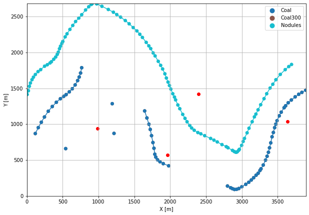
Plotting the Orientations#
[26]:
fig, ax = plt.subplots(1, figsize=(10, 10))

interfaces.plot(ax=ax, column='formation', legend=True, aspect='equal')
interfaces_coords.plot(ax=ax, column='formation', legend=True, aspect='equal')
orientations.plot(ax=ax, color='red', aspect='equal')
plt.grid()
ax.set_xlabel('X [m]')
ax.set_ylabel('Y [m]')
ax.set_xlim(0, 3892)
ax.set_ylim(0, 2683)
[26]:
(0.0, 2683.0)
GemPy Model Construction#
The structural geological model will be constructed using the GemPy package.
[27]:
import gempy as gp
WARNING (theano.configdefaults): g++ not available, if using conda: `conda install m2w64-toolchain`
WARNING (theano.configdefaults): g++ not detected ! Theano will be unable to execute optimized C-implementations (for both CPU and GPU) and will default to Python implementations. Performance will be severely degraded. To remove this warning, set Theano flags cxx to an empty string.
WARNING (theano.tensor.blas): Using NumPy C-API based implementation for BLAS functions.
Creating new Model#
[28]:
geo_model = gp.create_model('Model17')
geo_model
[28]:
Model17 2022-04-05 11:11
Initiate Data#
[29]:
gp.init_data(geo_model, [0, 3892, 0, 2683, 0, 1000], [100, 100, 100],
             surface_points_df=interfaces_coords[interfaces_coords['Z'] != 0],
             orientations_df=orientations,
             default_values=True)
Active grids: ['regular']
[29]:
Model17 2022-04-05 11:11
Model Surfaces#
[30]:
geo_model.surfaces
[30]:
| surface | series | order_surfaces | color | id | |
|---|---|---|---|---|---|
| 0 | Coal300 | Default series | 1 | #015482 | 1 |
| 1 | Coal | Default series | 2 | #9f0052 | 2 |
| 2 | Nodules | Default series | 3 | #ffbe00 | 3 |
Mapping the Stack to Surfaces#
[31]:
gp.map_stack_to_surfaces(geo_model,
                         {
                          'Strata1': ('Coal300', 'Coal', 'Nodules'),
                         },
                         remove_unused_series=True)
geo_model.add_surfaces('Basement')
[31]:
| surface | series | order_surfaces | color | id | |
|---|---|---|---|---|---|
| 0 | Coal300 | Strata1 | 1 | #015482 | 1 |
| 1 | Coal | Strata1 | 2 | #9f0052 | 2 |
| 2 | Nodules | Strata1 | 3 | #ffbe00 | 3 |
| 3 | Basement | Strata1 | 4 | #728f02 | 4 |
Showing the Number of Data Points#
[32]:
gg.utils.show_number_of_data_points(geo_model=geo_model)
[32]:
| surface | series | order_surfaces | color | id | No. of Interfaces | No. of Orientations | |
|---|---|---|---|---|---|---|---|
| 0 | Coal300 | Strata1 | 1 | #015482 | 1 | 69 | 0 |
| 1 | Coal | Strata1 | 2 | #9f0052 | 2 | 69 | 3 |
| 2 | Nodules | Strata1 | 3 | #ffbe00 | 3 | 103 | 1 |
| 3 | Basement | Strata1 | 4 | #728f02 | 4 | 0 | 0 |
Loading Digital Elevation Model#
[33]:
geo_model.set_topography(
    source='gdal', filepath=file_path + 'raster17.tif')
Cropped raster to geo_model.grid.extent.
depending on the size of the raster, this can take a while...
storing converted file...
Active grids: ['regular' 'topography']
[33]:
Grid Object. Values:
array([[  19.46      ,   13.415     ,    5.        ],
       [  19.46      ,   13.415     ,   15.        ],
       [  19.46      ,   13.415     ,   25.        ],
       ...,
       [3886.99742931, 2657.97201493,  594.15032959],
       [3886.99742931, 2667.98320896,  593.5199585 ],
       [3886.99742931, 2677.99440299,  592.91101074]])
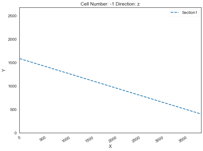
Defining Custom Section#
[34]:
custom_section = gpd.read_file(file_path + 'customsection17.shp')
custom_section_dict = gg.utils.to_section_dict(custom_section, section_column='name')
geo_model.set_section_grid(custom_section_dict)
Active grids: ['regular' 'topography' 'sections']
[34]:
| start | stop | resolution | dist | |
|---|---|---|---|---|
| Section1 | [6.648494638704051, 1585.9987115807176] | [3888.2970423641327, 402.8423753990243] | [100, 80] | 4057.96 |
[35]:
gp.plot.plot_section_traces(geo_model)
[35]:
<gempy.plot.visualization_2d.Plot2D at 0x18708b29ac0>
Plotting Input Data#
[36]:
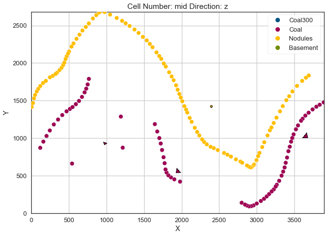
gp.plot_2d(geo_model, direction='z', show_lith=False, show_boundaries=False)
plt.grid()
[37]:
gp.plot_3d(geo_model, image=False, plotter_type='basic', notebook=True)
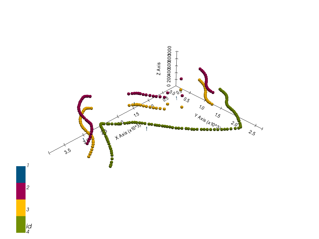
[37]:
<gempy.plot.vista.GemPyToVista at 0x187073560a0>
Setting the Interpolator#
[38]:
gp.set_interpolator(geo_model,
                    compile_theano=True,
                    theano_optimizer='fast_compile',
                    verbose=[],
                    update_kriging=False
                    )
Compiling theano function...
Level of Optimization:  fast_compile
Device:  cpu
Precision:  float64
Number of faults:  0
Compilation Done!
Kriging values:
                    values
range             4831.79
$C_o$           555860.79
drift equations       [3]
[38]:
<gempy.core.interpolator.InterpolatorModel at 0x18706891c70>
Computing Model#
[39]:
sol = gp.compute_model(geo_model, compute_mesh=True)
Plotting Cross Sections#
[40]:
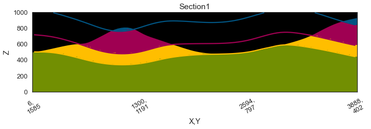
gp.plot_2d(geo_model, section_names=['Section1'], show_topography=True, show_data=False)
[40]:
<gempy.plot.visualization_2d.Plot2D at 0x1870b8fa760>
[41]:
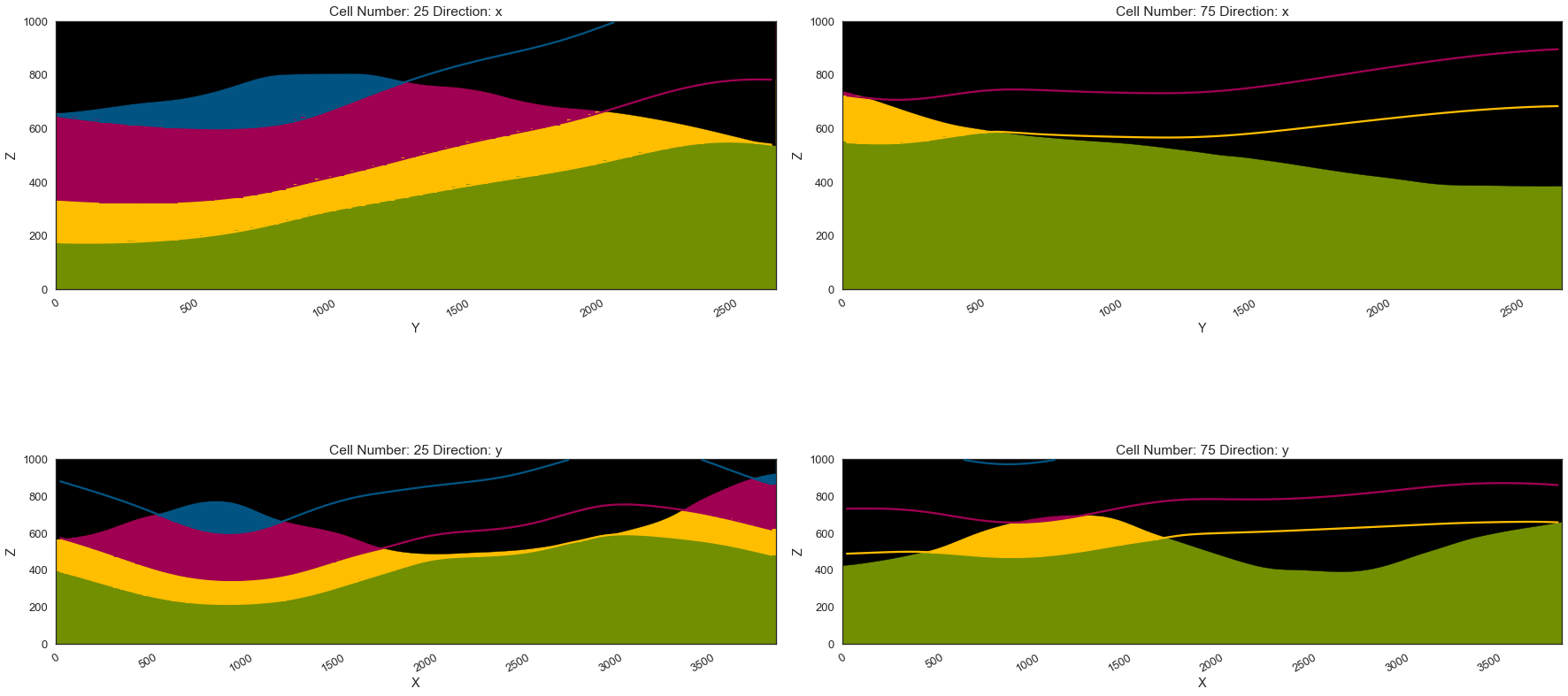
gp.plot_2d(geo_model, direction=['x', 'x', 'y', 'y'], cell_number=[25, 75, 25, 75], show_topography=True, show_data=False)
[41]:
<gempy.plot.visualization_2d.Plot2D at 0x187089cd670>
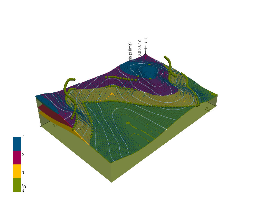
Plotting 3D Model#
[42]:
gpv = gp.plot_3d(geo_model, image=False, show_topography=True,
                 plotter_type='basic', notebook=True, show_lith=True)
[ ]: