55 Extracting Well Tops from PyVista Meshes

The following notebook illustrates how to extract well tops or in the case of GemPy well bases from PyVista meshes of GemPy models. In particular, a ray tracing algorithm in PyVista is used to extract the intersections of a borehole (PyVista Polydata) with a PyVista mesh. Straight boreholes as well as deviated boreholes can be used.

Set File Paths and download Tutorial Data

If you downloaded the latest GemGIS version from the Github repository, append the path so that the package can be imported successfully. Otherwise, it is recommended to install GemGIS via pip install gemgis and import GemGIS using import gemgis as gg. In addition, the file path to the folder where the data is being stored is set. The tutorial data is downloaded using Pooch (https://www.fatiando.org/pooch/latest/index.html) and stored in the specified folder. Use pip install pooch if Pooch is not installed on your system yet.

import warnings
warnings.filterwarnings("ignore")
import gemgis as gg
import geopandas as gpd
import rasterio
import gempy as gp
import pyvista as pv
import matplotlib.pyplot as plt
import numpy as np
import pandas as pd

WARNING (theano.configdefaults): g++ not available, if using conda: `conda install m2w64-toolchain`
WARNING (theano.configdefaults): g++ not detected ! Theano will be unable to execute optimized C-implementations (for both CPU and GPU) and will default to Python implementations. Performance will be severely degraded. To remove this warning, set Theano flags cxx to an empty string.
WARNING (theano.tensor.blas): Using NumPy C-API based implementation for BLAS functions.

file_path ='data/55_extracting_well_tops_from_pyvista_meshes/'
gg.download_gemgis_data.download_tutorial_data(filename="55_extracting_well_tops_from_pyvista_meshes.zip", dirpath=file_path)

Creating GemPy Model

Loading Topography

topo_raster = rasterio.open(file_path + 'raster1.tif')

Creating Interfaces

interfaces = gpd.read_file(file_path + 'interfaces1_lines.shp')
interfaces_coords = gg.vector.extract_xyz(gdf=interfaces, dem=topo_raster)
interfaces_coords.head()

	formation	geometry	X	Y	Z
0	Sand1	POINT (0.256 264.862)	0.26	264.86	353.97
1	Sand1	POINT (10.593 276.734)	10.59	276.73	359.04
2	Sand1	POINT (17.135 289.090)	17.13	289.09	364.28
3	Sand1	POINT (19.150 293.313)	19.15	293.31	364.99
4	Sand1	POINT (27.795 310.572)	27.80	310.57	372.81

Creating Orientations

orientations = gpd.read_file(file_path + 'orientations1.shp')
orientations = gg.vector.extract_xyz(gdf=orientations, dem=topo_raster)
orientations['polarity'] = 1
orientations

	formation	dip	azimuth	geometry	X	Y	Z	polarity
0	Ton	30.50	180.00	POINT (96.471 451.564)	96.47	451.56	440.59	1
1	Ton	30.50	180.00	POINT (172.761 661.877)	172.76	661.88	556.38	1
2	Ton	30.50	180.00	POINT (383.074 957.758)	383.07	957.76	729.02	1
3	Ton	30.50	180.00	POINT (592.356 722.702)	592.36	722.70	601.55	1
4	Ton	30.50	180.00	POINT (766.586 348.469)	766.59	348.47	378.63	1
5	Ton	30.50	180.00	POINT (843.907 167.023)	843.91	167.02	282.61	1
6	Ton	30.50	180.00	POINT (941.846 428.883)	941.85	428.88	423.45	1
7	Ton	30.50	180.00	POINT (22.142 299.553)	22.14	299.55	368.05	1

Calculating GemPy Model

geo_model = gp.create_model('Model1')
gp.init_data(geo_model, [0, 972, 0, 1069, 300, 800], [50, 50, 50],
             surface_points_df=interfaces_coords,
             orientations_df=orientations,
             default_values=True)
gp.map_stack_to_surfaces(geo_model,
                         {'Strata': ('Sand1', 'Ton')},
                         remove_unused_series=True)
geo_model.add_surfaces('Basement')
geo_model.set_topography(source='gdal', filepath=file_path + 'raster1.tif')
gp.set_interpolator(geo_model,
                    compile_theano=True,
                    theano_optimizer='fast_compile',
                    verbose=[],
                    update_kriging=False
                    )
sol = gp.compute_model(geo_model, compute_mesh=True)

Active grids: ['regular']
Cropped raster to geo_model.grid.extent.
depending on the size of the raster, this can take a while...
storing converted file...
Active grids: ['regular' 'topography']
Compiling theano function...
Level of Optimization:  fast_compile
Device:  cpu
Precision:  float64
Number of faults:  0
Compilation Done!
Kriging values:
                   values
range             1528.9
$C_o$           55655.83
drift equations      [3]

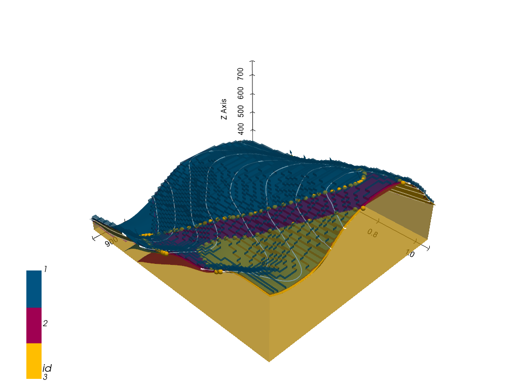
gpv = gp.plot_3d(geo_model,
                 image=False,
                 show_topography=True,
                 plotter_type='basic',
                 notebook=True,
                 show_lith=True,
                 show_boundaries=True)

Extracting Surfaces from the GemPy Model

mesh = gg.visualization.create_depth_maps_from_gempy(geo_model=geo_model, surfaces=['Sand1', 'Ton'])
mesh

{'Sand1': [PolyData (0x1e4a0b2b3a0)
    N Cells:    4209
    N Points:   2325
    X Bounds:   9.720e+00, 9.623e+02
    Y Bounds:   1.672e+02, 9.497e+02
    Z Bounds:   3.050e+02, 7.250e+02
    N Arrays:   1,
  '#015482'],
 'Ton': [PolyData (0x1e49c0c30a0)
    N Cells:    5396
    N Points:   2891
    X Bounds:   9.720e+00, 9.623e+02
    Y Bounds:   2.799e+02, 1.058e+03
    Z Bounds:   3.050e+02, 7.297e+02
    N Arrays:   1,
  '#9f0052']}

Extracting intersections between boreholes and meshes

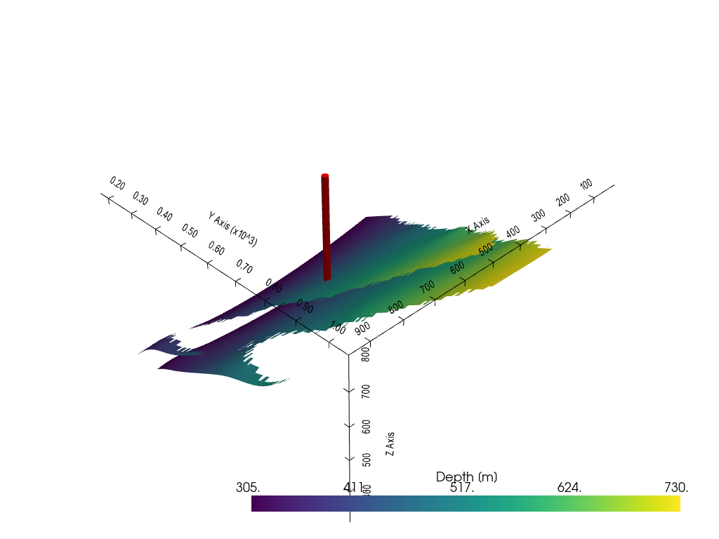
First, a PolyData set is created and visualized. The first attempt shows a straight vertical well.

well = pv.Line((500,500, 800), (500, 500, 300))
well_tube = well.tube(radius=10)
well_tube

Header	Data Arrays
PolyData Information N Cells 22 N Points 80 X Bounds 4.900e+02, 5.100e+02 Y Bounds 4.900e+02, 5.100e+02 Z Bounds 3.000e+02, 8.000e+02 N Arrays 3	Name Field Type N Comp Min Max Texture Coordinates Points float32 2 0.000e+00 1.000e+00 Distance Points float64 1 0.000e+00 5.000e+02 TubeNormals Points float32 3 -1.000e+00 1.000e+00

p = pv.Plotter(notebook=True)

p.add_mesh(mesh['Sand1'][0], scalars = 'Depth [m]')
p.add_mesh(mesh['Ton'][0], scalars = 'Depth [m]')
p.add_mesh(well_tube, color='red')
p.show_bounds()
p.show()

gg.utils.ray_trace_one_surface(mesh['Sand1'][0],
                               well.points[0],
                               well.points[1])

(array([[500.     , 500.     , 465.47574]], dtype=float32), array([2895]))

gg.utils.ray_trace_multiple_surfaces([mesh['Sand1'][0], mesh['Ton'][0]],
                                      well.points[0],
                                      well.points[1])

[(array([[500.     , 500.     , 465.47574]], dtype=float32), array([2895])),
 (array([[500.     , 500.     , 408.50534]], dtype=float32), array([3181]))]

gg.utils.create_virtual_profile(names_surfaces=list(mesh.keys()),
                                surfaces=[mesh['Sand1'][0], mesh['Ton'][0]],
                                borehole=well)

	Surface	Z
0	Sand1	465.48
1	Ton	408.51

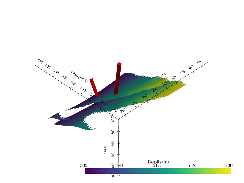
The second test will be made with a not so much realistic well path but to illustrate that also deviated boreholes work to extract the intersections. Here, we define a well with three segments (four points).

points = np.array(((500,600, 800),
                   (500, 550, 460),
                   (500, 350, 300),
                   (500, 250, 500)))

polyline = polyline_from_points(points)
tube = polyline.tube(radius=15)
polyline

Header	Data Arrays
PolyData Information N Cells 1 N Points 4 X Bounds 5.000e+02, 5.000e+02 Y Bounds 2.500e+02, 6.000e+02 Z Bounds 3.000e+02, 8.000e+02 N Arrays 1	Name Field Type N Comp Min Max scalars Points int32 1 0.000e+00 3.000e+00

p = pv.Plotter(notebook=True)

p.add_mesh(mesh['Sand1'][0], scalars = 'Depth [m]')
p.add_mesh(mesh['Ton'][0], scalars = 'Depth [m]')
p.add_mesh(tube, color='red')
p.show_bounds()
p.show()

gg.utils.create_virtual_profile(names_surfaces=list(mesh.keys()),
                                surfaces=[mesh['Sand1'][0], mesh['Ton'][0]],
                                borehole=polyline)

	Surface	Z
0	Sand1	497.21
1	Ton	377.33
2	Sand1	357.01
3	Ton	313.96