66 Generating Voronoi Polygons

This notebook illustrates the creation of Thiessen Polygons to illustrate the the data quantity of borehole data according to page 236 of the following report of the BGE: https://www.bge.de/fileadmin/user_upload/Standortsuche/Wesentliche_Unterlagen/Methodik/Phase_I_Schritt_2/rvSU-Methodik/20220328_Anlage_zu_rvSU_Konzept_Methodenbeschreibung_barrierefrei.pdf

Set File Paths and download Tutorial Data

If you downloaded the latest GemGIS version from the Github repository, append the path so that the package can be imported successfully. Otherwise, it is recommended to install GemGIS via pip install gemgis and import GemGIS using import gemgis as gg. In addition, the file path to the folder where the data is being stored is set. The tutorial data is downloaded using Pooch (https://www.fatiando.org/pooch/latest/index.html) and stored in the specified folder. Use pip install pooch if Pooch is not installed on your system yet.

import warnings
warnings.filterwarnings("ignore")

import gemgis as gg
import geopandas as gpd
import matplotlib.pyplot as plt

file_path ='data/66_generating_voronoi_polygons/'
# gg.download_gemgis_data.download_tutorial_data(filename="66_generating_voronoi_polygons.zip", dirpath=file_path)

Loading Borehole Data

The borehole data was extracted from the borehole database of the Geological Survey of NRW (https://www.gd.nrw.de/gd_archive_dabo.htm).

data = gpd.read_file(file_path + 'Bohrungen_groesser_1000.shp')
data.head()

	Index	DABO No.	Name	Number	Depth	X	Y	Z	X_GK	Y_GK	...	Kind	Procedure	Confidenti	Record Typ	Lithlog Ve	Quality	Drilling P	Remarks	Availabili	geometry
0	GD10092	DABO_102029	Klingerhuf1(1982)	NaN	1118.00	32332544.77	5701554.56	30.80	2541103.04	5700806.87	...	Bohrung	gemischtes Bohrverfahren	offen; Bohrung mit dokumentiertem Freigabeverm...	Übertragung eines alten Archivbestandes	1	Schichtdaten von guter Qualität; genaue strati...	30.9.1982 - 1.12.1982	Karbon Cumulus	Original-Schichtenverzeichnis liegt vor	POINT (32332544.770 5701554.560)
1	GD50035	DABO_1521	Salzbergen2	NaN	1875.70	32388961.53	5798219.66	30.00	2593500.00	5799735.00	...	Bohrung	gemischtes Bohrverfahren	vertraulich, offen nur mit Einwilligung; Eigen...	Aufnahme durch Sachbearbeiter; überarbeitet na...	1	Schichtdaten von guter Qualität; genaue strati...	15.2.1949 - 27.5.1950	paläontologisch untersucht; Ausführliche Unter...	Original-Schichtenverzeichnis liegt vor	POINT (32388961.530 5798219.660)
2	GD50073	DABO_1564	B.Salzbergen3	3	1908.90	32390628.91	5799824.32	36.00	2595100.00	5801408.00	...	Bohrung	Spülbohrung (Rotary-Verfahren)	vertraulich, offen nur mit Einwilligung; Eigen...	Übertragung eines alten Archivbestandes	1	Schichtdaten von guter Qualität; genaue strati...	19.10.1950 - 25.5.1951	siehe Original-Schichtenverzeichnis	Original-Schichtenverzeichnis liegt vor	POINT (32390628.910 5799824.320)
3	GD50261	DABO_2319	Ibbenbüren-Westfeld1	UB1121	1352.00	32409115.65	5798184.48	118.20	3409152.00	5800063.00	...	Bohrung	gemischtes Bohrverfahren	offen; Bohrung mit dokumentiertem Freigabeverm...	Übertragung eines alten Archivbestandes	1	Schichtdaten von guter Qualität; genaue strati...	11.11.1974 - 14.1.1975	Karbon Cumulus	Original-Schichtenverzeichnis liegt vor	POINT (32409115.650 5798184.480)
4	GD51096	DABO_7331	GildehausZ1	NaN	1683.10	32370464.85	5790221.74	40.00	2575345.00	5790975.00	...	Bohrung	gemischtes Bohrverfahren	vertraulich, offen nur mit Einwilligung; Eigen...	Aufnahme durch Sachbearbeiter; überarbeitet na...	1	Schichtdaten von guter Qualität; genaue strati...	..1956	Ausführliche Unterlagen im Original	Original-Schichtenverzeichnis liegt vor	POINT (32370464.850 5790221.740)

5 rows × 26 columns

Loading the Outline of NRW

outline = gpd.read_file(file_path + 'outline.shp')
outline

	osm_id	class	type	name	address	extratags	geometry
0	62761.00	boundary	administrative	North Rhine-Westphalia, Germany	"state"=>"North Rhine-Westphalia","ISO3166-2-l...	"ref:nuts"=>"DEA","wikidata"=>"Q1198","wikiped...	MULTIPOLYGON (((300636.227 5600913.724, 300639...

outline.crs

<Projected CRS: EPSG:25832>
Name: ETRS89 / UTM zone 32N
Axis Info [cartesian]:
- E[east]: Easting (metre)
- N[north]: Northing (metre)
Area of Use:
- name: Europe between 6°E and 12°E: Austria; Belgium; Denmark - onshore and offshore; Germany - onshore and offshore; Norway including - onshore and offshore; Spain - offshore.
- bounds: (6.0, 38.76, 12.01, 84.33)
Coordinate Operation:
- name: UTM zone 32N
- method: Transverse Mercator
Datum: European Terrestrial Reference System 1989 ensemble
- Ellipsoid: GRS 1980
- Prime Meridian: Greenwich

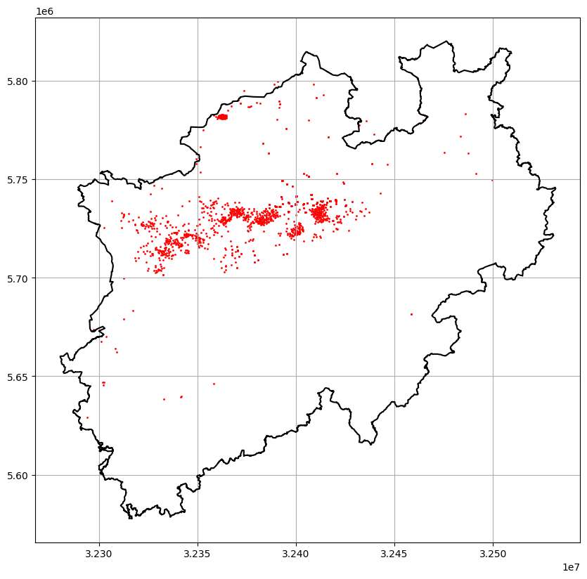
Plotting the Borehole Data

fig, ax = plt.subplots(1, figsize=(10,10))

outline.to_crs('EPSG:4647').boundary.plot(ax=ax, color='black')
data.plot(ax=ax, markersize=1, color='red')

plt.grid()

Voronoi Tessalation

gdf = gg.vector.create_voronoi_polygons(data)
gdf

	geometry	area
0	POLYGON ((32473194.081 5718253.741, 32469287.8...	665698318.29
1	POLYGON ((32473175.498 5773862.463, 32481354.2...	184545066.31
2	POLYGON ((32481354.247 5765667.587, 32481234.9...	304148453.73
3	POLYGON ((32459819.403 5765274.413, 32473175.4...	490884327.21
4	POLYGON ((32317260.014 5640927.969, 32314568.7...	250801576.02
...	...	...
1131	POLYGON ((32326629.143 5727191.374, 32326669.3...	922649.29
1132	POLYGON ((32326895.182 5726701.188, 32327147.6...	1407420.98
1133	POLYGON ((32327531.454 5727716.570, 32327549.9...	349756.27
1134	POLYGON ((32327677.535 5727156.396, 32328944.7...	1725230.07
1135	POLYGON ((32327531.454 5727716.570, 32327549.9...	3340904.68

1135 rows × 2 columns

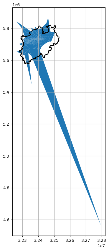
Plotting Valid Voronoi Polygons

fig, ax = plt.subplots(1, figsize=(10,10))

gdf.plot(ax=ax)
outline.to_crs('EPSG:4647').boundary.plot(ax=ax, color='black')

plt.grid()
plt.show()

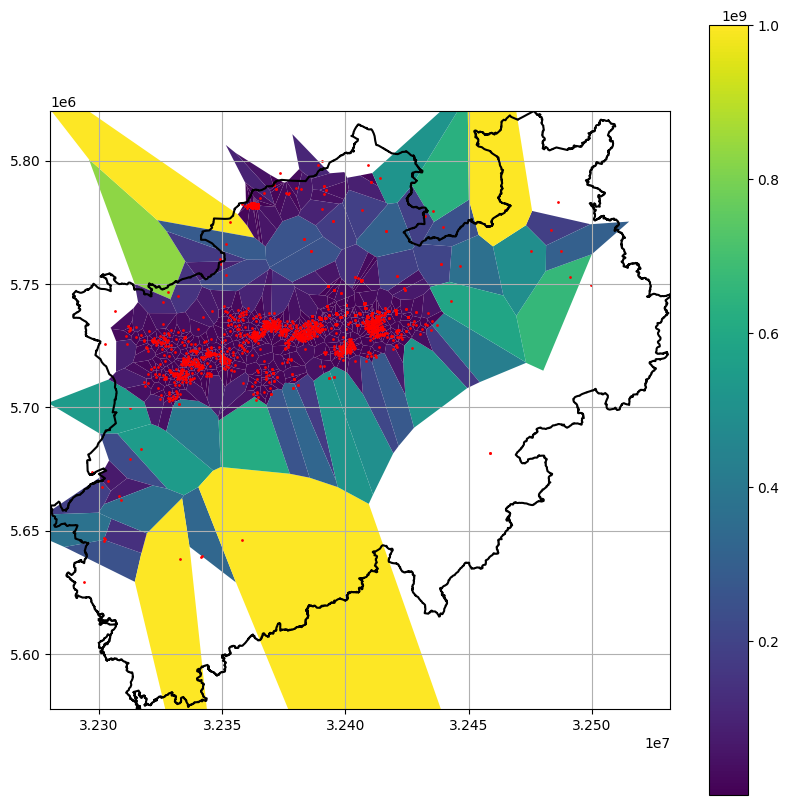
Plotting GeoDataFrame

fig, ax = plt.subplots(1, figsize=(10,10))

outline.to_crs('EPSG:4647').boundary.plot(ax=ax, color='black')#
gdf.plot(ax=ax, column='area', vmax=1e9, legend=True)
data.plot(ax=ax, markersize=1, color='red')

plt.xlim(outline.to_crs('EPSG:4647').total_bounds[0], outline.to_crs('EPSG:4647').total_bounds[2])
plt.ylim(outline.to_crs('EPSG:4647').total_bounds[1], outline.to_crs('EPSG:4647').total_bounds[3])
plt.grid()
plt.show()