19 Working with Web Map Services - WMS
Contents
19 Working with Web Map Services - WMS#
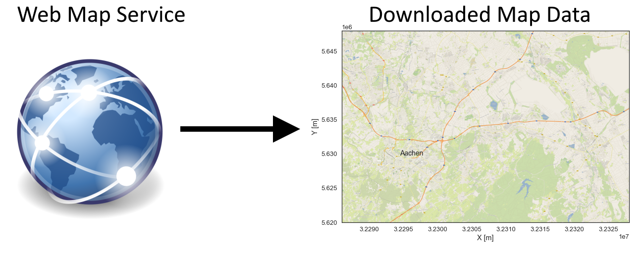
A Web Map Service (WMS) is a standard protocol developed by the Open Geospatial Consortium in 1999 for serving georeferenced map images over the Internet. These images are typically produced by a map server from data provided by a GIS database.
The map information can be downloaded as map data and stored as array for further usage.
Source: https://en.wikipedia.org/wiki/Web_Map_Service
Set File Paths and download Tutorial Data#
If you downloaded the latest GemGIS version from the Github repository, append the path so that the package can be imported successfully. Otherwise, it is recommended to install GemGIS via pip install gemgis and import GemGIS using import gemgis as gg. In addition, the file path to the folder where the data is being stored is set. The tutorial data is downloaded using Pooch (https://www.fatiando.org/pooch/latest/index.html) and stored in the specified folder. Use
pip install pooch if Pooch is not installed on your system yet.
[2]:
import gemgis as gg

file_path ='data/19_working_with_web_map_services/'
WARNING (theano.configdefaults): g++ not available, if using conda: `conda install m2w64-toolchain`
C:\Users\ale93371\Anaconda3\envs\test_gempy\lib\site-packages\theano\configdefaults.py:560: UserWarning: DeprecationWarning: there is no c++ compiler.This is deprecated and with Theano 0.11 a c++ compiler will be mandatory
  warnings.warn("DeprecationWarning: there is no c++ compiler."
WARNING (theano.configdefaults): g++ not detected ! Theano will be unable to execute optimized C-implementations (for both CPU and GPU) and will default to Python implementations. Performance will be severely degraded. To remove this warning, set Theano flags cxx to an empty string.
WARNING (theano.tensor.blas): Using NumPy C-API based implementation for BLAS functions.
Loading the Web Map Service#
Loading the Web Map Service from https://ows.terrestris.de/.
[2]:
wms = gg.web.load_wms(url='https://ows.terrestris.de/osm/service?')
wms
WARNING (theano.configdefaults): g++ not available, if using conda: `conda install m2w64-toolchain`
C:\Users\ale93371\Anaconda3\envs\test_gempy\lib\site-packages\theano\configdefaults.py:560: UserWarning: DeprecationWarning: there is no c++ compiler.This is deprecated and with Theano 0.11 a c++ compiler will be mandatory
  warnings.warn("DeprecationWarning: there is no c++ compiler."
WARNING (theano.configdefaults): g++ not detected ! Theano will be unable to execute optimized C-implementations (for both CPU and GPU) and will default to Python implementations. Performance will be severely degraded. To remove this warning, set Theano flags cxx to an empty string.
WARNING (theano.tensor.blas): Using NumPy C-API based implementation for BLAS functions.
[2]:
<owslib.map.wms111.WebMapService_1_1_1 at 0x261a7a250d0>
Checking the type of the WMS#
[3]:
wms.identification.type
[3]:
'OGC:WMS'
Checking the version of the WMS#
[4]:
wms.identification.version
[4]:
'1.1.1'
Checking the title of the WMS#
[5]:
wms.identification.title
[5]:
'OpenStreetMap WMS'
Checking the abstract of the WMS#
[6]:
wms.identification.abstract
[6]:
'OpenStreetMap WMS, bereitgestellt durch terrestris GmbH und Co. KG. Beschleunigt mit MapProxy (http://mapproxy.org/)'
Checking the operations of the WMS#
[7]:
wms.getOperationByName('GetMap').methods
[7]:
[{'type': 'Get', 'url': 'https://ows.terrestris.de/osm/service?'}]
Checking the format options of the WMS#
[8]:
# The different formats a layer can be saved as
wms.getOperationByName('GetMap').formatOptions
[8]:
['image/jpeg', 'image/png']
Checking the title of a WMS layer#
[9]:
# Title of a layer
wms['OSM-WMS'].title
[9]:
'OpenStreetMap WMS - by terrestris'
Checking the CRS options of a WMS layer#
[10]:
# Available CRS systems for a layer
wms['OSM-WMS'].crsOptions
[10]:
['EPSG:25833',
 'EPSG:4326',
 'EPSG:29192',
 'EPSG:32648',
 'EPSG:5243',
 'EPSG:4674',
 'EPSG:4686',
 'EPSG:900913',
 'EPSG:2056',
 'EPSG:31466',
 'EPSG:4258',
 'EPSG:2180',
 'EPSG:2100',
 'EPSG:21781',
 'EPSG:29193',
 'EPSG:31463',
 'EPSG:3068',
 'EPSG:31467',
 'EPSG:4647',
 'EPSG:4839',
 'EPSG:31468',
 'EPSG:3857',
 'EPSG:25832',
 'EPSG:3034',
 'EPSG:3035']
Checking the styles of the WMS Layer#
[11]:
# Available styles
wms['OSM-WMS'].styles
[11]:
{'default': {'title': 'default',
  'legend': 'https://ows.terrestris.de/osm/service?styles=&layer=OSM-WMS&service=WMS&format=image%2Fpng&sld_version=1.1.0&request=GetLegendGraphic&version=1.1.1'}}
Checking the bounding box of the WMS layer#
[12]:
wms['OSM-WMS'].boundingBox
[12]:
(-20037508.3428, -25819498.5135, 20037508.3428, 25819498.5135, 'EPSG:900913')
Checking the bounding box of the WMS layer#
[13]:
wms['OSM-WMS'].boundingBoxWGS84
[13]:
(-180.0, -88.0, 180.0, 88.0)
[14]:
wms['OSM-WMS'].opaque
[14]:
0
[15]:
wms['OSM-WMS'].queryable
[15]:
1
Getting map data for the WMS layer#
[16]:
wms_map = gg.web.load_as_map(url=wms.url,
                             layer='OSM-WMS',
                             style='default',
                             crs='EPSG:4647',
                             bbox=[32286000,32328000, 5620000,5648000],
                             size=[4200, 2800],
                             filetype='image/png')
[17]:
wms_map
[17]:
<owslib.util.ResponseWrapper at 0x261d348cc10>
Converting the map data to an array#
[18]:
# Converting WMS map object to array
import io
import matplotlib.pyplot as plt

maps = io.BytesIO(wms_map.read())
wms_array = plt.imread(maps)
wms_array[:1]
[18]:
array([[[0.8039216 , 0.7647059 , 0.65882355],
        [0.85882354, 0.8784314 , 0.6627451 ],
        [0.87058824, 0.91764706, 0.6666667 ],
        ...,
        [0.78431374, 0.7647059 , 0.65882355],
        [0.8862745 , 0.9019608 , 0.81960785],
        [0.9529412 , 0.93333334, 0.9019608 ]]], dtype=float32)
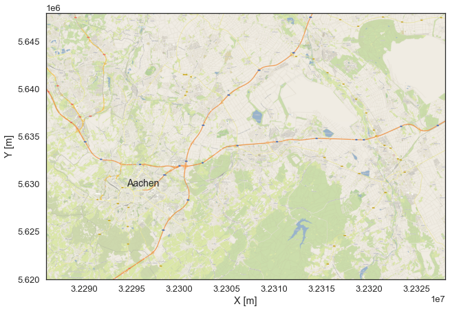
Getting the array data for the WMS layer#
This layer shows the OpenStreet Map data for the Aachen area.
[19]:
wms_array = gg.web.load_as_array(url=wms.url,
                                 layer='OSM-WMS',
                                 style='default',
                                 crs='EPSG:4647',
                                 bbox=[32286000,32328000, 5620000,5648000],
                                 size=[4200, 2800],
                                 filetype='image/png')

wms_array[:1]
[19]:
array([[[0.8039216 , 0.7647059 , 0.65882355],
        [0.85882354, 0.8784314 , 0.6627451 ],
        [0.87058824, 0.91764706, 0.6666667 ],
        ...,
        [0.78431374, 0.7647059 , 0.65882355],
        [0.8862745 , 0.9019608 , 0.81960785],
        [0.9529412 , 0.93333334, 0.9019608 ]]], dtype=float32)
Plotting the map data#
[20]:
plt.imshow(wms_array, extent=[32286000, 32328000,5620000,5648000])
plt.xlabel('X [m]')
plt.ylabel('Y [m]')
plt.text(32294500,5629750, 'Aachen', size = 14)
[20]:
Text(32294500, 5629750, 'Aachen')
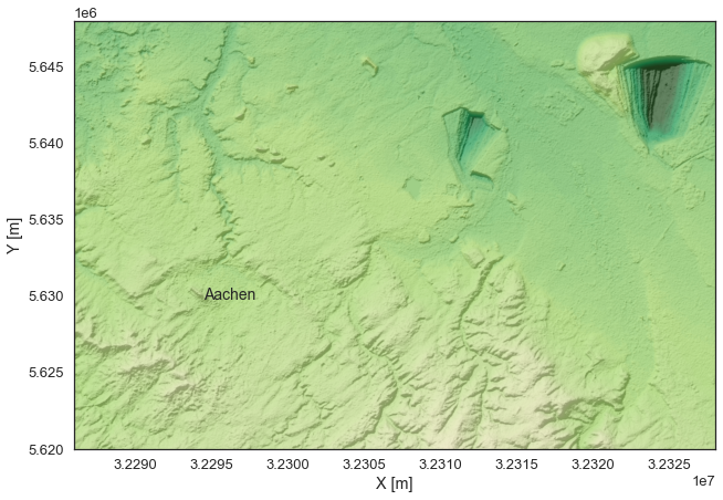
Getting map data for the WMS layer#
This layer shows the hillshades of the Aachen area together with a colored digital elevation model.
[21]:
wms_array = gg.web.load_as_array(url=wms.url,
                                 layer='SRTM30-Colored-Hillshade',
                                 style='default',
                                 crs='EPSG:4647',
                                 bbox=[32286000,32328000, 5620000,5648000],
                                 size=[4200, 2800],
                                 filetype='image/png')

wms_array[:1]
[21]:
array([[[0.56078434, 0.77254903, 0.5137255 , 1.        ],
        [0.54901963, 0.7607843 , 0.5019608 , 1.        ],
        [0.5568628 , 0.76862746, 0.5058824 , 1.        ],
        ...,
        [0.49411765, 0.7490196 , 0.5058824 , 1.        ],
        [0.49411765, 0.7490196 , 0.5058824 , 1.        ],
        [0.49803922, 0.7529412 , 0.50980395, 1.        ]]], dtype=float32)
Plotting the map data#
[22]:
plt.imshow(wms_array, extent=[32286000, 32328000,5620000,5648000])
plt.xlabel('X [m]')
plt.ylabel('Y [m]')
plt.text(32294500,5629750, 'Aachen', size = 14)
[22]:
Text(32294500, 5629750, 'Aachen')
Checking the data#
[23]:
wms_array[:1]
[23]:
array([[[0.56078434, 0.77254903, 0.5137255 , 1.        ],
        [0.54901963, 0.7607843 , 0.5019608 , 1.        ],
        [0.5568628 , 0.76862746, 0.5058824 , 1.        ],
        ...,
        [0.49411765, 0.7490196 , 0.5058824 , 1.        ],
        [0.49411765, 0.7490196 , 0.5058824 , 1.        ],
        [0.49803922, 0.7529412 , 0.50980395, 1.        ]]], dtype=float32)
Loading the WMS#
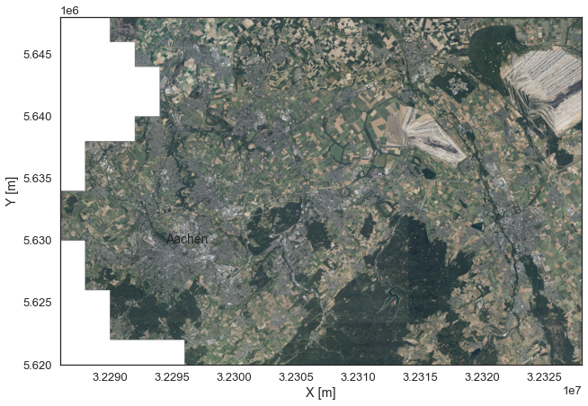
The next layer represents orthophotos of the Aachen area.
[24]:
wms = gg.web.load_wms('https://www.wms.nrw.de/geobasis/wms_nw_dop')
wms
[24]:
<owslib.map.wms111.WebMapService_1_1_1 at 0x261d53bed60>
Getting map data for the WMS layer#
[25]:
wms_array = gg.web.load_as_array(url=wms.url,
                                 layer='nw_dop_rgb',
                                 style='default',
                                 crs='EPSG:4647',
                                 bbox=[32286000,32328000, 5620000,5648000],
                                 size=[4200, 2800],
                                 filetype='image/png')

wms_array[:1]
[25]:
array([[[0.        , 0.        , 0.        , 0.        ],
        [0.        , 0.        , 0.        , 0.        ],
        [0.        , 0.        , 0.        , 0.        ],
        ...,
        [0.29803923, 0.33333334, 0.3137255 , 1.        ],
        [0.3019608 , 0.33333334, 0.32941177, 1.        ],
        [0.2901961 , 0.3019608 , 0.2901961 , 1.        ]]], dtype=float32)
Plotting the map data#
[26]:
plt.imshow(wms_array, extent=[32286000, 32328000,5620000,5648000])
plt.xlabel('X [m]')
plt.ylabel('Y [m]')
plt.text(32294500,5629750, 'Aachen', size = 14)
[26]:
Text(32294500, 5629750, 'Aachen')
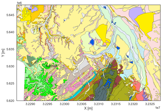
Loading the WMS#
The next layer is the geological map of the Aachen area.
[27]:
wms = gg.web.load_wms('http://www.wms.nrw.de/gd/GK100')
wms
[27]:
<owslib.map.wms111.WebMapService_1_1_1 at 0x261d53d8280>
Getting map data for the WMS layer#
[28]:
wms_array = gg.web.load_as_array(url=wms.url,
                                 layer='0',
                                 style='default',
                                 crs='EPSG:4647',
                                 bbox=[32286000,32328000, 5620000,5648000],
                                 size=[1400,933],
                                 filetype='image/png')

wms_array[:1]
[28]:
array([[[0.9882353 , 0.87058824, 0.87058824, 1.        ],
        [0.9882353 , 0.87058824, 0.87058824, 1.        ],
        [0.9882353 , 0.87058824, 0.87058824, 1.        ],
        ...,
        [0.99607843, 0.9607843 , 0.6039216 , 1.        ],
        [0.99607843, 0.9607843 , 0.6039216 , 1.        ],
        [0.99607843, 0.9607843 , 0.6039216 , 1.        ]]], dtype=float32)
Plotting the map data#
[29]:
plt.imshow(wms_array, extent=[32286000, 32328000,5620000,5648000])
plt.xlabel('X [m]')
plt.ylabel('Y [m]')
plt.text(32294500,5629750, 'Aachen', size = 14)
[29]:
Text(32294500, 5629750, 'Aachen')