
Example 21 - Coal Seam Mining
Contents
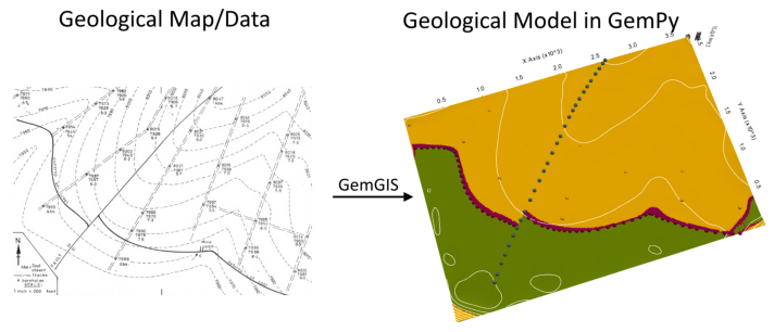
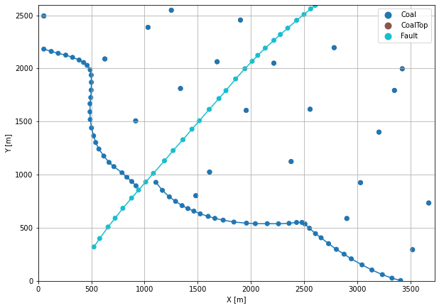
Example 21 - Coal Seam Mining#
This example will show how to convert the geological map below using GemGIS to a GemPy model. This example is based on digitized data. The area is 3727 m wide (W-E extent) and 2596 m high (N-S extent). The vertical model extent varies between 2400 m and 2475 m. The model represents a coal seam that is outcropping at the surface and was encountered in boreholes at depth.
The map has been georeferenced with QGIS. The stratigraphic boundaries were digitized in QGIS. Strikes lines were digitized in QGIS as well and will be used to calculate orientations for the GemPy model. The contour lines were also digitized and will be interpolated with GemGIS to create a topography for the model.
Map Source: An Introduction to Geological Structures and Maps by G.M. Bennison
[1]:
import matplotlib.pyplot as plt
import matplotlib.image as mpimg
img = mpimg.imread('../images/cover_example21.png')
plt.figure(figsize=(10, 10))
imgplot = plt.imshow(img)
plt.axis('off')
plt.tight_layout()
Licensing#
Computational Geosciences and Reservoir Engineering, RWTH Aachen University, Authors: Alexander Juestel. For more information contact: alexander.juestel(at)rwth-aachen.de
This work is licensed under a Creative Commons Attribution 4.0 International License (http://creativecommons.org/licenses/by/4.0/)
Import GemGIS#
If you have installed GemGIS via pip and conda, you can import GemGIS like any other package. If you have downloaded the repository, append the path to the directory where the GemGIS repository is stored and then import GemGIS.
[2]:
import warnings
warnings.filterwarnings("ignore")
import gemgis as gg
Importing Libraries and loading Data#
All remaining packages can be loaded in order to prepare the data and to construct the model. The example data is downloaded from an external server using pooch. It will be stored in a data folder in the same directory where this notebook is stored.
[3]:
import geopandas as gpd
import rasterio
[4]:
file_path = 'data/example21/'
gg.download_gemgis_data.download_tutorial_data(filename="example21_coal_seam_mining.zip", dirpath=file_path)
Downloading file 'example21_coal_seam_mining.zip' from 'https://rwth-aachen.sciebo.de/s/AfXRsZywYDbUF34/download?path=%2Fexample21_coal_seam_mining.zip' to 'C:\Users\ale93371\Documents\gemgis\docs\getting_started\example\data\example21'.
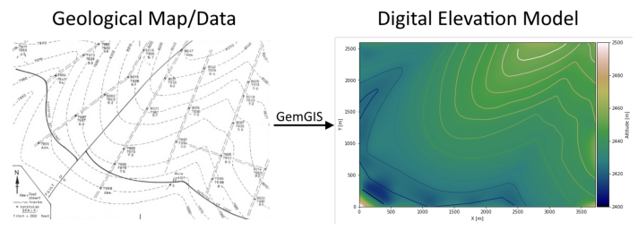
Creating Digital Elevation Model from Contour Lines#
The digital elevation model (DEM) will be created by interpolating contour lines digitized from the georeferenced map using the SciPy Radial Basis Function interpolation wrapped in GemGIS. The respective function used for that is gg.vector.interpolate_raster().
[5]:
import matplotlib.pyplot as plt
import matplotlib.image as mpimg
img = mpimg.imread('../images/dem_example21.png')
plt.figure(figsize=(10, 10))
imgplot = plt.imshow(img)
plt.axis('off')
plt.tight_layout()
[6]:
topo = gpd.read_file(file_path + 'topo21.shp')
topo['Z'] = topo['Z']*0.3048
topo.head()
[6]:
| id | Z | geometry | |
|---|---|---|---|
| 0 | None | 2423.16 | LINESTRING (8.426 1648.306, 35.717 1675.998, 6... |
| 1 | None | 2426.21 | LINESTRING (5.215 1950.921, 79.464 1983.831, 1... |
| 2 | None | 2429.26 | LINESTRING (16.854 2215.007, 64.213 2217.014, ... |
| 3 | None | 2432.30 | LINESTRING (24.179 2563.075, 70.835 2554.346, ... |
| 4 | None | 2432.30 | LINESTRING (957.912 2594.380, 1031.960 2594.98... |
Interpolating the contour lines#
[7]:
topo_raster = gg.vector.interpolate_raster(gdf=topo, value='Z', method='rbf', res=10)
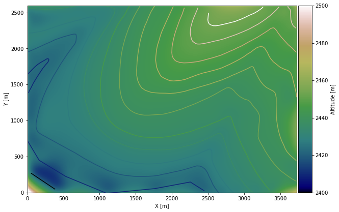
Plotting the raster#
[8]:
import matplotlib.pyplot as plt

from mpl_toolkits.axes_grid1 import make_axes_locatable

fix, ax = plt.subplots(1, figsize=(10, 10))
topo.plot(ax=ax, aspect='equal', column='Z', cmap='gist_earth')
im = ax.imshow(topo_raster, origin='lower', extent=[0, 3727, 0, 2596], cmap='gist_earth', clim=[2400, 2500])
divider = make_axes_locatable(ax)
cax = divider.append_axes("right", size="5%", pad=0.05)
cbar = plt.colorbar(im, cax=cax)
cbar.set_label('Altitude [m]')
ax.set_xlabel('X [m]')
ax.set_ylabel('Y [m]')
ax.set_xlim(0, 3727)
ax.set_ylim(0, 2596)
[8]:
(0.0, 2596.0)
Saving the raster to disc#
After the interpolation of the contour lines, the raster is saved to disc using gg.raster.save_as_tiff(). The function will not be executed as a raster is already provided with the example data.
Opening Raster#
The previously computed and saved raster can now be opened using rasterio.
[9]:
topo_raster = rasterio.open(file_path + 'raster21.tif')
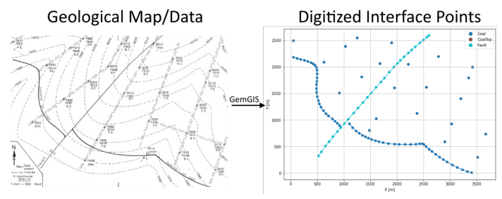
Interface Points of stratigraphic boundaries#
The interface points will be extracted from LineStrings digitized from the georeferenced map using QGIS. It is important to provide a formation name for each layer boundary. The vertical position of the interface point will be extracted from the digital elevation model using the GemGIS function gg.vector.extract_xyz(). The resulting GeoDataFrame now contains single points including the information about the respective formation.
[10]:
import matplotlib.pyplot as plt
import matplotlib.image as mpimg
img = mpimg.imread('../images/interfaces_example21.png')
plt.figure(figsize=(10, 10))
imgplot = plt.imshow(img)
plt.axis('off')
plt.tight_layout()
[11]:
interfaces = gpd.read_file(file_path + 'interfaces21.shp')
interfaces.head()
[11]:
| id | formation | geometry | |
|---|---|---|---|
| 0 | None | Coal | LINESTRING (53.076 2181.695, 122.910 2160.023,... |
| 1 | None | Coal | LINESTRING (1107.213 927.687, 1168.017 852.435... |
| 2 | None | Fault | LINESTRING (523.855 319.647, 578.639 399.114, ... |
Extracting Z coordinate from Digital Elevation Model#
[12]:
interfaces_coords = gg.vector.extract_xyz(gdf=interfaces, dem=topo_raster)
interfaces_coords = interfaces_coords.sort_values(by='formation', ascending=False)
interfaces_coords.head()
[12]:
| formation | geometry | X | Y | Z | |
|---|---|---|---|---|---|
| 87 | Fault | POINT (2604.437 2592.875) | 2604.44 | 2592.88 | 2458.99 |
| 73 | Fault | POINT (1608.696 1614.592) | 1608.70 | 1614.59 | 2442.26 |
| 59 | Fault | POINT (523.855 319.647) | 523.86 | 319.65 | 2422.09 |
| 60 | Fault | POINT (578.639 399.114) | 578.64 | 399.11 | 2424.08 |
| 61 | Fault | POINT (657.504 507.477) | 657.50 | 507.48 | 2425.55 |
[13]:
boreholes = gpd.read_file(file_path + 'points21.shp')
boreholes = gg.vector.extract_xy(gdf=boreholes)
boreholes['Z'] = boreholes['Z']*0.3048
boreholes.head()
[13]:
| formation | Z | geometry | X | Y | |
|---|---|---|---|---|---|
| 0 | CoalTop | 2421.64 | POINT (627.403 2088.984) | 627.40 | 2088.98 |
| 1 | CoalTop | 2426.21 | POINT (53.076 2493.542) | 53.08 | 2493.54 |
| 2 | CoalTop | 2416.45 | POINT (1033.164 2386.382) | 1033.16 | 2386.38 |
| 3 | CoalTop | 2414.02 | POINT (1252.300 2547.724) | 1252.30 | 2547.72 |
| 4 | CoalTop | 2425.29 | POINT (916.975 1506.229) | 916.97 | 1506.23 |
[14]:
import pandas as pd
interfaces_coords = pd.concat([interfaces_coords, boreholes])
interfaces_coords = interfaces_coords[interfaces_coords['formation'].isin(['Fault', 'CoalTop', 'Coal'])].reset_index()
interfaces_coords
[14]:
| index | formation | geometry | X | Y | Z | |
|---|---|---|---|---|---|---|
| 0 | 87 | Fault | POINT (2604.437 2592.875) | 2604.44 | 2592.88 | 2458.99 |
| 1 | 73 | Fault | POINT (1608.696 1614.592) | 1608.70 | 1614.59 | 2442.26 |
| 2 | 59 | Fault | POINT (523.855 319.647) | 523.86 | 319.65 | 2422.09 |
| 3 | 60 | Fault | POINT (578.639 399.114) | 578.64 | 399.11 | 2424.08 |
| 4 | 61 | Fault | POINT (657.504 507.477) | 657.50 | 507.48 | 2425.55 |
| ... | ... | ... | ... | ... | ... | ... |
| 127 | 39 | Coal | POINT (3204.651 1400.273) | 3204.65 | 1400.27 | 2416.45 |
| 128 | 40 | Coal | POINT (3350.340 1792.790) | 3350.34 | 1792.79 | 2411.88 |
| 129 | 41 | Coal | POINT (3423.787 1996.273) | 3423.79 | 1996.27 | 2409.75 |
| 130 | 42 | Coal | POINT (3520.110 293.760) | 3520.11 | 293.76 | 2429.87 |
| 131 | 43 | Coal | POINT (3673.023 733.235) | 3673.02 | 733.23 | 2424.68 |
132 rows × 6 columns
Plotting the Interface Points#
[15]:
fig, ax = plt.subplots(1, figsize=(10, 10))

interfaces.plot(ax=ax, column='formation', legend=True, aspect='equal')
interfaces_coords.plot(ax=ax, column='formation', legend=True, aspect='equal')
plt.grid()
ax.set_xlabel('X [m]')
ax.set_ylabel('Y [m]')
ax.set_xlim(0, 3727)
ax.set_ylim(0, 2596)
[15]:
(0.0, 2596.0)
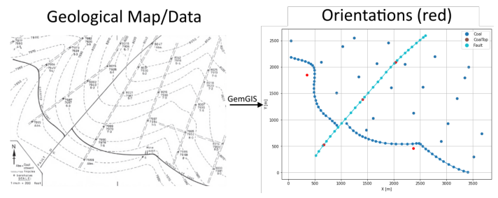
Orientations from Strike Lines#
Strike lines connect outcropping stratigraphic boundaries (interfaces) of the same altitude. In other words: the intersections between topographic contours and stratigraphic boundaries at the surface. The height difference and the horizontal difference between two digitized lines is used to calculate the dip and azimuth and hence an orientation that is necessary for GemPy. In order to calculate the orientations, each set of strikes lines/LineStrings for one formation must be given an id
number next to the altitude of the strike line. The id field is already predefined in QGIS. The strike line with the lowest altitude gets the id number 1, the strike line with the highest altitude the the number according to the number of digitized strike lines. It is currently recommended to use one set of strike lines for each structural element of one formation as illustrated.
[16]:
import matplotlib.pyplot as plt
import matplotlib.image as mpimg
img = mpimg.imread('../images/orientations_example21.png')
plt.figure(figsize=(10, 10))
imgplot = plt.imshow(img)
plt.axis('off')
plt.tight_layout()
[17]:
strikes = gpd.read_file(file_path + 'strikes21.shp')
strikes['Z'] = strikes['Z']*0.3048
strikes.head()
[17]:
| id | formation | Z | geometry | |
|---|---|---|---|---|
| 0 | 1 | Coal1 | 2426.21 | LINESTRING (335.423 2099.821, 499.173 1840.952) |
| 1 | 2 | Coal1 | 2429.26 | LINESTRING (564.191 1250.972, 3.108 2216.613) |
| 2 | 2 | Coal2 | 2432.30 | LINESTRING (1619.532 600.790, 2945.181 207.069) |
| 3 | 1 | Coal2 | 2429.26 | LINESTRING (2364.833 540.588, 2570.724 477.978) |
[18]:
orientations_fault = gpd.read_file(file_path + 'orientations21_fault.shp')
orientations_fault = gg.vector.extract_xyz(gdf=orientations_fault, dem=topo_raster)
orientations_fault
[18]:
| formation | dip | azimuth | polarity | geometry | X | Y | Z | |
|---|---|---|---|---|---|---|---|---|
| 0 | Fault | 60.00 | 305.00 | 1.00 | POINT (670.146 526.140) | 670.15 | 526.14 | 2425.71 |
| 1 | Fault | 60.00 | 305.00 | 1.00 | POINT (1410.631 1387.029) | 1410.63 | 1387.03 | 2439.39 |
| 2 | Fault | 60.00 | 305.00 | 1.00 | POINT (2034.324 2095.005) | 2034.32 | 2095.00 | 2447.71 |
Calculate Orientations for each formation#
[19]:
orientations_coal1 = gg.vector.calculate_orientations_from_strike_lines(gdf=strikes[strikes['formation'] == 'Coal1'].sort_values(by='Z', ascending=True).reset_index())
orientations_coal1
[19]:
| dip | azimuth | Z | geometry | polarity | formation | X | Y | |
|---|---|---|---|---|---|---|---|---|
| 0 | 0.76 | 59.69 | 2427.73 | POINT (350.474 1852.089) | 1.00 | Coal1 | 350.47 | 1852.09 |
[20]:
orientations_coal2 = gg.vector.calculate_orientations_from_strike_lines(gdf=strikes[strikes['formation'] == 'Coal2'].sort_values(by='Z', ascending=True).reset_index())
orientations_coal2
[20]:
| dip | azimuth | Z | geometry | polarity | formation | X | Y | |
|---|---|---|---|---|---|---|---|---|
| 0 | 1.14 | 16.55 | 2430.78 | POINT (2375.067 456.607) | 1.00 | Coal2 | 2375.07 | 456.61 |
Merging Orientations#
[21]:
import pandas as pd
orientations = pd.concat([orientations_coal1, orientations_coal2, orientations_fault]).reset_index()
orientations['formation'] = ['Coal', 'Coal', 'Fault', 'Fault', 'Fault']
orientations = orientations[orientations['formation'].isin(['Coal', 'Fault'])]
orientations
[21]:
| index | dip | azimuth | Z | geometry | polarity | formation | X | Y | |
|---|---|---|---|---|---|---|---|---|---|
| 0 | 0 | 0.76 | 59.69 | 2427.73 | POINT (350.474 1852.089) | 1.00 | Coal | 350.47 | 1852.09 |
| 1 | 0 | 1.14 | 16.55 | 2430.78 | POINT (2375.067 456.607) | 1.00 | Coal | 2375.07 | 456.61 |
| 2 | 0 | 60.00 | 305.00 | 2425.71 | POINT (670.146 526.140) | 1.00 | Fault | 670.15 | 526.14 |
| 3 | 1 | 60.00 | 305.00 | 2439.39 | POINT (1410.631 1387.029) | 1.00 | Fault | 1410.63 | 1387.03 |
| 4 | 2 | 60.00 | 305.00 | 2447.71 | POINT (2034.324 2095.005) | 1.00 | Fault | 2034.32 | 2095.00 |
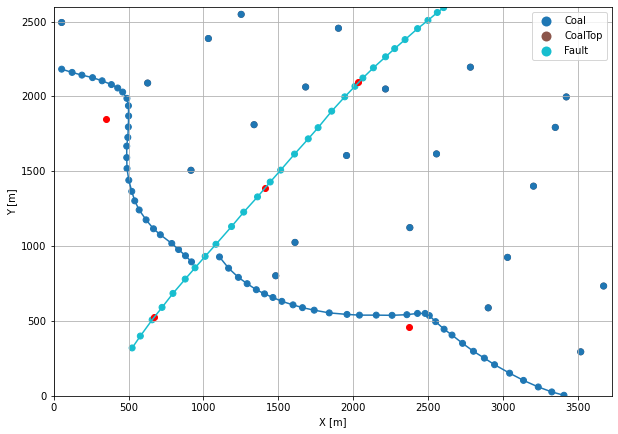
Plotting the Orientations#
[22]:
fig, ax = plt.subplots(1, figsize=(10, 10))

interfaces.plot(ax=ax, column='formation', legend=True, aspect='equal')
interfaces_coords.plot(ax=ax, column='formation', legend=True, aspect='equal')
orientations.plot(ax=ax, color='red', aspect='equal')
plt.grid()
ax.set_xlabel('X [m]')
ax.set_ylabel('Y [m]')
ax.set_xlim(0, 3727)
ax.set_ylim(0, 2596)
[22]:
(0.0, 2596.0)
GemPy Model Construction#
The structural geological model will be constructed using the GemPy package.
[23]:
import gempy as gp
WARNING (theano.configdefaults): g++ not available, if using conda: `conda install m2w64-toolchain`
WARNING (theano.configdefaults): g++ not detected ! Theano will be unable to execute optimized C-implementations (for both CPU and GPU) and will default to Python implementations. Performance will be severely degraded. To remove this warning, set Theano flags cxx to an empty string.
WARNING (theano.tensor.blas): Using NumPy C-API based implementation for BLAS functions.
Creating new Model#
[24]:
geo_model = gp.create_model('Model21')
geo_model
[24]:
Model21 2022-04-05 11:19
Initiate Data#
[25]:
gp.init_data(geo_model, [0, 3727, 0, 2596, 2400, 2475], [100, 100, 100],
             surface_points_df=interfaces_coords[interfaces_coords['Z'] != 0],
             orientations_df=orientations,
             default_values=True)
Active grids: ['regular']
[25]:
Model21 2022-04-05 11:19
Model Surfaces#
[26]:
geo_model.surfaces
[26]:
| surface | series | order_surfaces | color | id | |
|---|---|---|---|---|---|
| 0 | Fault | Default series | 1 | #015482 | 1 |
| 1 | Coal | Default series | 2 | #9f0052 | 2 |
| 2 | CoalTop | Default series | 3 | #ffbe00 | 3 |
Mapping the Stack to Surfaces#
[27]:
gp.map_stack_to_surfaces(geo_model,
                         {
                          'Fault1': ('Fault'),
                          'Strata1': ('CoalTop', 'Coal'),
                         },
                         remove_unused_series=True)
geo_model.add_surfaces('Basement')
geo_model.set_is_fault(['Fault1'])
Fault colors changed. If you do not like this behavior, set change_color to False.
[27]:
| order_series | BottomRelation | isActive | isFault | isFinite | |
|---|---|---|---|---|---|
| Fault1 | 1 | Fault | True | True | False |
| Strata1 | 2 | Erosion | True | False | False |
Showing the Number of Data Points#
[28]:
gg.utils.show_number_of_data_points(geo_model=geo_model)
[28]:
| surface | series | order_surfaces | color | id | No. of Interfaces | No. of Orientations | |
|---|---|---|---|---|---|---|---|
| 0 | Fault | Fault1 | 1 | #527682 | 1 | 29 | 3 |
| 1 | Coal | Strata1 | 1 | #9f0052 | 2 | 81 | 2 |
| 2 | CoalTop | Strata1 | 2 | #ffbe00 | 3 | 22 | 0 |
| 3 | Basement | Strata1 | 3 | #728f02 | 4 | 0 | 0 |
Loading Digital Elevation Model#
[29]:
geo_model.set_topography(
    source='gdal', filepath=file_path + 'raster21.tif')
Cropped raster to geo_model.grid.extent.
depending on the size of the raster, this can take a while...
storing converted file...
Active grids: ['regular' 'topography']
[29]:
Grid Object. Values:
array([[  18.635     ,   12.98      , 2400.375     ],
       [  18.635     ,   12.98      , 2401.125     ],
       [  18.635     ,   12.98      , 2401.875     ],
       ...,
       [3722.04388298, 2571.13409962, 2462.30371094],
       [3722.04388298, 2581.08045977, 2463.51391602],
       [3722.04388298, 2591.02681992, 2464.8894043 ]])
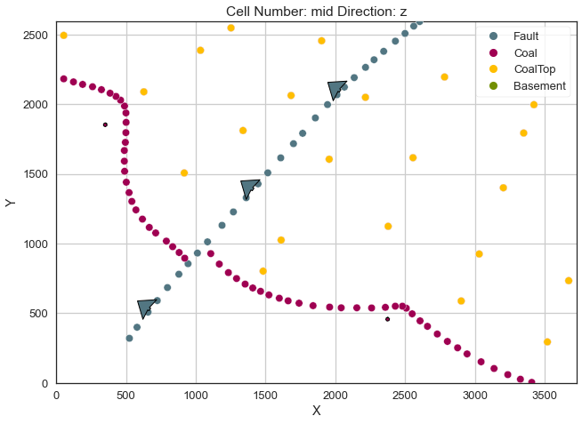
Plotting Input Data#
[30]:
gp.plot_2d(geo_model, direction='z', show_lith=False, show_boundaries=False)
plt.grid()
[31]:
gp.plot_3d(geo_model, image=False, plotter_type='basic', notebook=True)
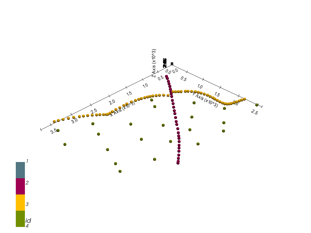
[31]:
<gempy.plot.vista.GemPyToVista at 0x1799e93afa0>
Setting the Interpolator#
[32]:
gp.set_interpolator(geo_model,
                    compile_theano=True,
                    theano_optimizer='fast_compile',
                    verbose=[],
                    update_kriging=False
                    )
Compiling theano function...
Level of Optimization:  fast_compile
Device:  cpu
Precision:  float64
Number of faults:  1
Compilation Done!
Kriging values:
                    values
range             4542.62
$C_o$           491318.33
drift equations    [3, 3]
[32]:
<gempy.core.interpolator.InterpolatorModel at 0x17997fa6520>
Computing Model#
[33]:
sol = gp.compute_model(geo_model, compute_mesh=True)
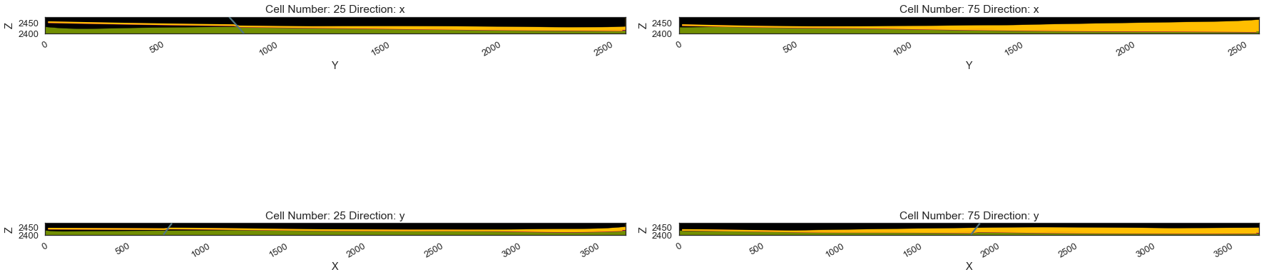
Plotting Cross Sections#
[34]:
gp.plot_2d(geo_model, direction=['x', 'x', 'y', 'y'], cell_number=[25, 75, 25, 75], show_topography=True, show_data=False)
[34]:
<gempy.plot.visualization_2d.Plot2D at 0x1799fb532b0>
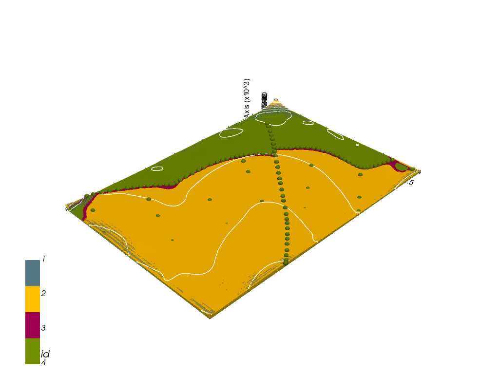
Plotting 3D Model#
[35]:
gpv = gp.plot_3d(geo_model, image=False, show_topography=True,
                 plotter_type='basic', notebook=True, show_lith=True)
[ ]: