42 Draping LineStrings over Digital Elevation Model in PyVista
Contents
42 Draping LineStrings over Digital Elevation Model in PyVista#
When displaying LineString data in combination with a Digital Elevation Model, it is desired to map LineStrings representing elements such as roads on top of the Digital Elevation Model instead of above or below. Here it is shown how to do that with GemGIS.
Set File Paths and download Tutorial Data#
If you downloaded the latest GemGIS version from the Github repository, append the path so that the package can be imported successfully. Otherwise, it is recommended to install GemGIS via pip install gemgis and import GemGIS using import gemgis as gg. In addition, the file path to the folder where the data is being stored is set. The tutorial data is downloaded using Pooch (https://www.fatiando.org/pooch/latest/index.html) and stored in the specified folder. Use
pip install pooch if Pooch is not installed on your system yet.
[1]:
import gemgis as gg

file_path ='data/42_draping_linestrings_over_dem_in_pyvista/'
[2]:
gg.download_gemgis_data.download_tutorial_data(filename="42_draping_linestrings_over_dem_in_pyvista.zip", dirpath=file_path)
Loading Mesh and Vector Data#
The loaded digital elevation model will be used under Datenlizenz Deutschland – Zero – Version 2.0. It was obtained from the WCS Service https://www.wcs.nrw.de/geobasis/wcs_nw_dgm.
[3]:
import pyvista as pv
import rasterio

raster = rasterio.open(file_path + 'DEM50_EPSG_4647_clipped.tif')

topo = pv.read(file_path + 'topo.vtk')
topo
[3]:
| Header | Data Arrays | ||||||||||||||||||||||||||||
|---|---|---|---|---|---|---|---|---|---|---|---|---|---|---|---|---|---|---|---|---|---|---|---|---|---|---|---|---|---|
|
|
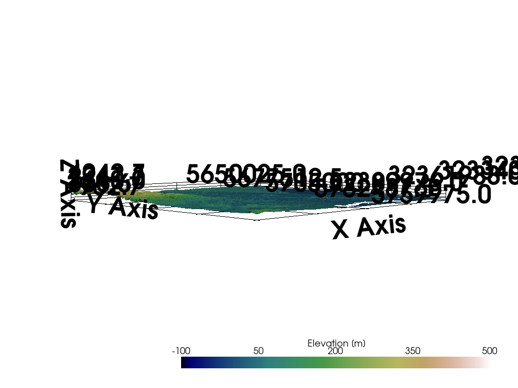
[4]:
import pyvista as pv

sargs = dict(fmt="%.0f", color='black')

p = pv.Plotter(notebook=True)

# Adding DEM
p.add_mesh(topo, scalars='Elevation [m]', cmap='gist_earth', scalar_bar_args=sargs, clim=[-100, 500])

p.set_background('white')
p.show_grid(color='black')
p.set_scale(1,1,10)
p.show()
C:\Users\ale93371\Anaconda3\envs\pygeomechanical\lib\site-packages\pyvista\jupyter\notebook.py:58: UserWarning: Failed to use notebook backend:

No module named 'trame'

Falling back to a static output.
  warnings.warn(
Creating 3D Line of County Boundary#
The boundary data was obtained from https://www.opengeodata.nrw.de/produkte/geobasis/vkg/dvg/dvg1/ and will be used under the same license as the Digital Elevation Model.
[5]:
import geopandas as gpd

boundary = gpd.read_file(file_path + 'dvg1rbz_nw.shp')
boundary = boundary[boundary['GN'] == 'Düsseldorf']
boundary.head()
[5]:
| ART | GN | KN | STAND | geometry | |
|---|---|---|---|---|---|
| 0 | R | Düsseldorf | 05100000 | 2020-03-04 | POLYGON ((295896.673 5747849.577, 295897.626 5... |
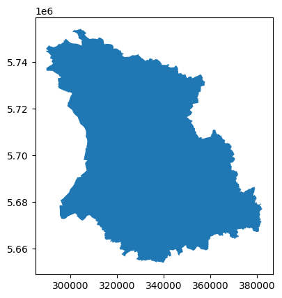
[6]:
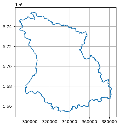
boundary.plot()
[6]:
<Axes: >
Exploding Polygon to LineString#
The first is to explode the polygon to a LineString using explode_polygons(..).
[7]:
boundary_line = gg.vector.explode_polygons(gdf=boundary)
boundary_line
[7]:
| ART | GN | KN | STAND | geometry | |
|---|---|---|---|---|---|
| 0 | R | Düsseldorf | 05100000 | 2020-03-04 | LINESTRING (295896.673 5747849.577, 295897.626... |
[8]:
import matplotlib.pyplot as plt

boundary_line.plot()
plt.grid()
Extracting vertices from line#
The next step is to extract the vertices from this one line using extract_xyz(..).
[9]:
boundary_points = gg.vector.extract_xyz(gdf=boundary_line, dem=raster, target_crs='EPSG:4647')
boundary_points
[9]:
| ART | GN | KN | STAND | geometry | X | Y | Z | |
|---|---|---|---|---|---|---|---|---|
| 0 | R | Düsseldorf | 05100000 | 2020-03-04 | POINT (32295896.673 5747849.577) | 32295896.67 | 5747849.58 | 11.49 |
| 1 | R | Düsseldorf | 05100000 | 2020-03-04 | POINT (32295897.626 5747850.839) | 32295897.63 | 5747850.84 | 11.56 |
| 2 | R | Düsseldorf | 05100000 | 2020-03-04 | POINT (32295943.179 5747880.192) | 32295943.18 | 5747880.19 | 11.44 |
| 3 | R | Düsseldorf | 05100000 | 2020-03-04 | POINT (32295959.070 5747891.749) | 32295959.07 | 5747891.75 | 11.70 |
| 4 | R | Düsseldorf | 05100000 | 2020-03-04 | POINT (32295975.984 5747906.266) | 32295975.98 | 5747906.27 | 11.55 |
| ... | ... | ... | ... | ... | ... | ... | ... | ... |
| 27446 | R | Düsseldorf | 05100000 | 2020-03-04 | POINT (32295802.571 5747693.901) | 32295802.57 | 5747693.90 | 11.58 |
| 27447 | R | Düsseldorf | 05100000 | 2020-03-04 | POINT (32295840.751 5747767.801) | 32295840.75 | 5747767.80 | 11.44 |
| 27448 | R | Düsseldorf | 05100000 | 2020-03-04 | POINT (32295857.959 5747796.720) | 32295857.96 | 5747796.72 | 11.65 |
| 27449 | R | Düsseldorf | 05100000 | 2020-03-04 | POINT (32295870.009 5747814.641) | 32295870.01 | 5747814.64 | 11.49 |
| 27450 | R | Düsseldorf | 05100000 | 2020-03-04 | POINT (32295896.673 5747849.577) | 32295896.67 | 5747849.58 | 11.49 |
27451 rows × 8 columns
Creating LineString with Z component#
A LineString with a Z component can be created using create_linestring_from_xyz_points(..).
[10]:
boundary_line_z = gg.vector.create_linestring_from_xyz_points(points=boundary_points)
boundary_line_z
[10]:

Creating GeoDataFrame from LineString#
[11]:
gdf_boundary = gpd.GeoDataFrame(geometry=[boundary_line_z])
gdf_boundary
[11]:
| geometry | |
|---|---|
| 0 | LINESTRING Z (32295896.673 5747849.577 11.490,... |
Creating 3D Lines#
The last step is to create the 3D lines and return the data as PyVista PolyData.
[12]:
boundary_pv = gg.visualization.create_lines_3d_polydata(gdf=gdf_boundary)
boundary_pv['Label'] = ['Regierungsbezirk Dusseldorf']
boundary_pv
[12]:
| Header | Data Arrays | ||||||||||||||||||||||||||||
|---|---|---|---|---|---|---|---|---|---|---|---|---|---|---|---|---|---|---|---|---|---|---|---|---|---|---|---|---|---|
|
|
Creating 3D lines of Faults#
The same workflow can be applied to a dataset with multiple LineStrings. In this case the faults that were mapped in the area.
[13]:
bbox = (32250000, 5650000, 32390000, 5760000)
[14]:
faults = gpd.read_file(file_path + 'gg_nrw_geotekst_l.shp', bbox=bbox)
faults.head()
[14]:
| OBJECTID_1 | OBJECTID_2 | Layer_Name | Quelle | ST_NAME | OBJECTID | Id | ssymbol_QB | ST_NR | ST_ART_ID | ... | DIP_3D | STOE_UEB_3 | STOE_TOP_H | STOE_BASIS | ST_ART_3D | Shape_Le_2 | Versatz_TB | Doku_Versa | Shape_Le_3 | geometry | |
|---|---|---|---|---|---|---|---|---|---|---|---|---|---|---|---|---|---|---|---|---|---|
| 0 | 52.00 | 52 | Störung040_Quadrather Sprung_SW | Erft Scholle RWE Projekt 2015 | Quadrather Sprung | 0 | 0 | NaN | 0.00 | 0 | ... | 62.50 | regionale Bedeutung | DGM | Tertiaer_b/Praeperm_t/Karbon_t | NaN | 9317.89 | 0.00 | NaN | 9317.89 | LINESTRING (32338164.037 5644376.205, 32338092... |
| 1 | 99.00 | 99 | Störung067_Peringshofer Sprung 1_NE | Erft Scholle RWE Projekt 2015 | Peringshofer Sprung | 0 | 0 | NaN | 0.00 | 0 | ... | 62.50 | lokale Bedeutung | DGM | Tertiaer_b/Praeperm_t/Karbon_t | NaN | 3304.34 | 0.00 | NaN | 3304.34 | LINESTRING (32332455.392 5650412.839, 32332407... |
| 2 | 100.00 | 100 | Störung068_Sandberg Sprung_NE | Erft Scholle RWE Projekt 2015 | Sandberg Sprung | 0 | 0 | NaN | 0.00 | 0 | ... | 62.50 | überregionale Bedeutung | DGM | Tertiaer_b/Praeperm_t/Karbon_t | NaN | 3242.54 | 0.00 | NaN | 3242.54 | LINESTRING (32331619.679 5651276.996, 32331513... |
| 3 | 101.00 | 101 | Störung069_Bedburger Sprung_NE | Erft Scholle RWE Projekt 2015 | Bedburger Sprung | 0 | 0 | NaN | 0.00 | 0 | ... | 62.50 | lokale Bedeutung | DGM | Tertiaer_b/Praeperm_t/Karbon_t | NaN | 6404.51 | 0.00 | NaN | 6404.51 | LINESTRING (32333471.001 5648319.956, 32333423... |
| 4 | 102.00 | 102 | Störung070_Bedburger Sprung 1_NE | Erft Scholle RWE Projekt 2015 | Bedburger Sprung | 0 | 0 | NaN | 0.00 | 0 | ... | 62.50 | lokale Bedeutung | DGM | Tertiaer_b/Praeperm_t/Karbon_t | NaN | 1656.99 | 0.00 | NaN | 1656.99 | LINESTRING (32332714.438 5649401.541, 32332618... |
5 rows × 47 columns
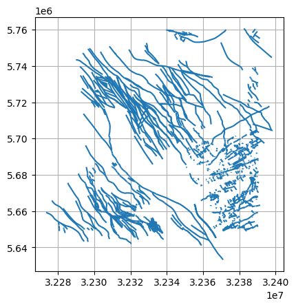
[15]:
import matplotlib.pyplot as plt

faults.plot()
plt.grid()
Extracting vertices from line#
The vertices will be extracted from the lines again. Here, it is important to NOT reset the index of the resulting GeoDataFrame!
[16]:
faults = faults[faults.is_valid]
faults = faults[~faults.is_empty]
faults = faults.explode().reset_index(drop=True)
faults_xyz = gg.vector.extract_xyz(gdf=faults, dem=raster, reset_index=False)
faults_xyz.head()
[16]:
| OBJECTID_1 | OBJECTID_2 | Layer_Name | Quelle | ST_NAME | OBJECTID | Id | ssymbol_QB | ST_NR | ST_ART_ID | ... | STOE_BASIS | ST_ART_3D | Shape_Le_2 | Versatz_TB | Doku_Versa | Shape_Le_3 | geometry | X | Y | Z | ||
|---|---|---|---|---|---|---|---|---|---|---|---|---|---|---|---|---|---|---|---|---|---|---|
| 0 | 0 | 52.00 | 52 | Störung040_Quadrather Sprung_SW | Erft Scholle RWE Projekt 2015 | Quadrather Sprung | 0 | 0 | NaN | 0.00 | 0 | ... | Tertiaer_b/Praeperm_t/Karbon_t | NaN | 9317.89 | 0.00 | NaN | 9317.89 | POINT (32338164.037 5644376.205) | 32338164.04 | 5644376.20 | 9999.00 |
| 0 | 52.00 | 52 | Störung040_Quadrather Sprung_SW | Erft Scholle RWE Projekt 2015 | Quadrather Sprung | 0 | 0 | NaN | 0.00 | 0 | ... | Tertiaer_b/Praeperm_t/Karbon_t | NaN | 9317.89 | 0.00 | NaN | 9317.89 | POINT (32338092.156 5644454.183) | 32338092.16 | 5644454.18 | 9999.00 | |
| 0 | 52.00 | 52 | Störung040_Quadrather Sprung_SW | Erft Scholle RWE Projekt 2015 | Quadrather Sprung | 0 | 0 | NaN | 0.00 | 0 | ... | Tertiaer_b/Praeperm_t/Karbon_t | NaN | 9317.89 | 0.00 | NaN | 9317.89 | POINT (32338020.275 5644532.162) | 32338020.28 | 5644532.16 | 9999.00 | |
| 0 | 52.00 | 52 | Störung040_Quadrather Sprung_SW | Erft Scholle RWE Projekt 2015 | Quadrather Sprung | 0 | 0 | NaN | 0.00 | 0 | ... | Tertiaer_b/Praeperm_t/Karbon_t | NaN | 9317.89 | 0.00 | NaN | 9317.89 | POINT (32337976.168 5644579.490) | 32337976.17 | 5644579.49 | 9999.00 | |
| 0 | 52.00 | 52 | Störung040_Quadrather Sprung_SW | Erft Scholle RWE Projekt 2015 | Quadrather Sprung | 0 | 0 | NaN | 0.00 | 0 | ... | Tertiaer_b/Praeperm_t/Karbon_t | NaN | 9317.89 | 0.00 | NaN | 9317.89 | POINT (32337847.430 5644717.324) | 32337847.43 | 5644717.32 | 9999.00 |
5 rows × 50 columns
Creating LineStrings with Z component#
As before, LineStrings with Z components will be created. This time, the function create_linestrings_from_xyz_points(..) is used.
[17]:
faults_lines_z = gg.vector.create_linestrings_from_xyz_points(gdf=faults_xyz, groupby='OBJECTID_2', return_gdf=True)
faults_lines_z
[17]:
| OBJECTID_1 | OBJECTID_2 | Layer_Name | Quelle | ST_NAME | OBJECTID | Id | ssymbol_QB | ST_NR | ST_ART_ID | ... | DIP_3D | STOE_UEB_3 | STOE_TOP_H | STOE_BASIS | ST_ART_3D | Shape_Le_2 | Versatz_TB | Doku_Versa | Shape_Le_3 | geometry | |
|---|---|---|---|---|---|---|---|---|---|---|---|---|---|---|---|---|---|---|---|---|---|
| 0 | 52.00 | 52 | Störung040_Quadrather Sprung_SW | Erft Scholle RWE Projekt 2015 | Quadrather Sprung | 0 | 0 | NaN | 0.00 | 0 | ... | 62.50 | regionale Bedeutung | DGM | Tertiaer_b/Praeperm_t/Karbon_t | NaN | 9317.89 | 0.00 | NaN | 9317.89 | LINESTRING Z (32332790.835 5650048.917 83.820,... |
| 1 | 99.00 | 99 | Störung067_Peringshofer Sprung 1_NE | Erft Scholle RWE Projekt 2015 | Peringshofer Sprung | 0 | 0 | NaN | 0.00 | 0 | ... | 62.50 | lokale Bedeutung | DGM | Tertiaer_b/Praeperm_t/Karbon_t | NaN | 3304.34 | 0.00 | NaN | 3304.34 | LINESTRING Z (32332455.392 5650412.839 69.640,... |
| 2 | 100.00 | 100 | Störung068_Sandberg Sprung_NE | Erft Scholle RWE Projekt 2015 | Sandberg Sprung | 0 | 0 | NaN | 0.00 | 0 | ... | 62.50 | überregionale Bedeutung | DGM | Tertiaer_b/Praeperm_t/Karbon_t | NaN | 3242.54 | 0.00 | NaN | 3242.54 | LINESTRING Z (32331619.679 5651276.996 54.820,... |
| 3 | 101.00 | 101 | Störung069_Bedburger Sprung_NE | Erft Scholle RWE Projekt 2015 | Bedburger Sprung | 0 | 0 | NaN | 0.00 | 0 | ... | 62.50 | lokale Bedeutung | DGM | Tertiaer_b/Praeperm_t/Karbon_t | NaN | 6404.51 | 0.00 | NaN | 6404.51 | LINESTRING Z (32331896.183 5650024.802 69.040,... |
| 4 | 102.00 | 102 | Störung070_Bedburger Sprung 1_NE | Erft Scholle RWE Projekt 2015 | Bedburger Sprung | 0 | 0 | NaN | 0.00 | 0 | ... | 62.50 | lokale Bedeutung | DGM | Tertiaer_b/Praeperm_t/Karbon_t | NaN | 1656.99 | 0.00 | NaN | 1656.99 | LINESTRING Z (32331991.560 5650081.463 69.630,... |
| ... | ... | ... | ... | ... | ... | ... | ... | ... | ... | ... | ... | ... | ... | ... | ... | ... | ... | ... | ... | ... | ... |
| 1510 | 13323.00 | 13324 | NaN | 3DLandesmodell | Hervester Sprung | 0 | 0 | NaN | 0.00 | 0 | ... | 79.00 | überregionale Bedeutung | Oberkreide_b | Praeperm_t/Karbon_t | NaN | 32201.82 | 0.00 | NaN | 32201.82 | LINESTRING Z (32372522.961 5716737.961 46.730,... |
| 1511 | 13324.00 | 13325 | NaN | 3DLandesmodell | Tertius Sprung | 0 | 0 | NaN | 0.00 | 0 | ... | 80.00 | überregionale Bedeutung | Oberkreide_b | Praeperm_t/Karbon_t | NaN | 45355.26 | 0.00 | NaN | 45355.26 | LINESTRING Z (32386330.289 5705646.290 88.140,... |
| 1512 | 13325.00 | 13326 | NaN | 3DLandesmodell | Rhader Stoerung | 0 | 0 | NaN | 0.00 | 0 | ... | 83.00 | überregionale Bedeutung | Oberkreide_b | Praeperm_t/Karbon_t | NaN | 50431.89 | 0.00 | NaN | 50431.89 | LINESTRING Z (32365258.965 5733746.961 52.790,... |
| 1513 | 13331.00 | 13332 | NaN | isgk100 | Bergische Überschiebung | 0 | 0 | NaN | 0.00 | 0 | ... | 80.00 | lokale Bedeutung | DGM | NaN | Abschiebung | 627.73 | 0.00 | NaN | 627.73 | LINESTRING Z (32372730.326 5650769.467 181.760... |
| 1514 | 13333.00 | 13334 | NaN | gk25_4707_Mettmann_Preußenkarte_Schriiver | NaN | 0 | 0 | NaN | 0.00 | 0 | ... | 0.00 | regionale Bedeutung | NaN | NaN | NaN | 7815.04 | 0.00 | NaN | 7815.04 | LINESTRING Z (32357075.547 5675077.272 82.920,... |
1515 rows × 47 columns
Creating 3D Lines#
The last step is to create the 3D lines and return the data as PyVista PolyData.
[19]:
faults_pv = gg.visualization.create_lines_3d_polydata(gdf=faults_lines_z)
faults_pv
[19]:
| PolyData | Information |
|---|---|
| N Cells | 1515 |
| N Points | 36539 |
| N Strips | 0 |
| X Bounds | 3.228e+07, 3.239e+07 |
| Y Bounds | 5.650e+06, 5.760e+06 |
| Z Bounds | -8.993e+01, 4.156e+02 |
| N Arrays | 0 |
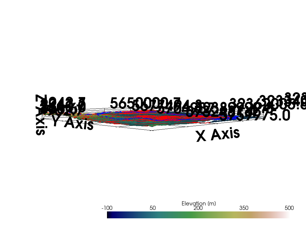
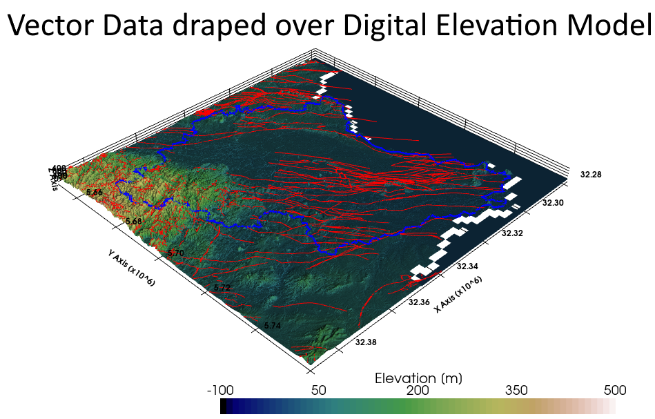
Plotting the data on top of the DEM#
[20]:
import pyvista as pv

sargs = dict(fmt="%.0f", color='black')

p = pv.Plotter(notebook=True)

# Adding DEM
p.add_mesh(topo, scalars='Elevation [m]', cmap='gist_earth', scalar_bar_args=sargs, clim=[-100, 500])

# Adding boundary
p.add_mesh(boundary_pv, color='blue', line_width=5)

# Adding faults
p.add_mesh(faults_pv,color='red', line_width=2)

p.set_background('white')
p.show_grid(color='black')
p.set_scale(1,1,10)
p.show()
C:\Users\ale93371\Anaconda3\envs\pygeomechanical\lib\site-packages\pyvista\jupyter\notebook.py:58: UserWarning: Failed to use notebook backend:

No module named 'trame'

Falling back to a static output.
  warnings.warn(